← All projects · Computer Vision · AI Engineering
Computer Vision
Muhammad Hammas · AI Engineer · Master's in Artificial Intelligence
Every project here produced a number or a figure on data it had not seen, and ships the code that produced it.
3D Vision
Open the page →Depth, surfaces, normals, registration and novel views. Classical methods and learned ones, measured against ground truth that is known in closed form or planted on purpose.
ICP registration
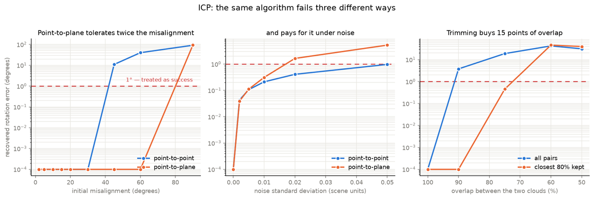
Point-to-plane tolerates twice the misalignment
Show the resultThe convergence basin is 30° for point-to-point and 60° for point-to-plane — exactly double. Past its basin ICP does not fail loudly; it converges confidently to the wrong alignment, which is why a residual cannot be used to detect the failure.
shape three fused blobs, 2,000 points — asymmetric, so rotation is unambiguous ground truth a known rigid transform; error is the geodesic angle to it varied initial misalignment, noise, overlap, trimming success recovered rotation within 1° 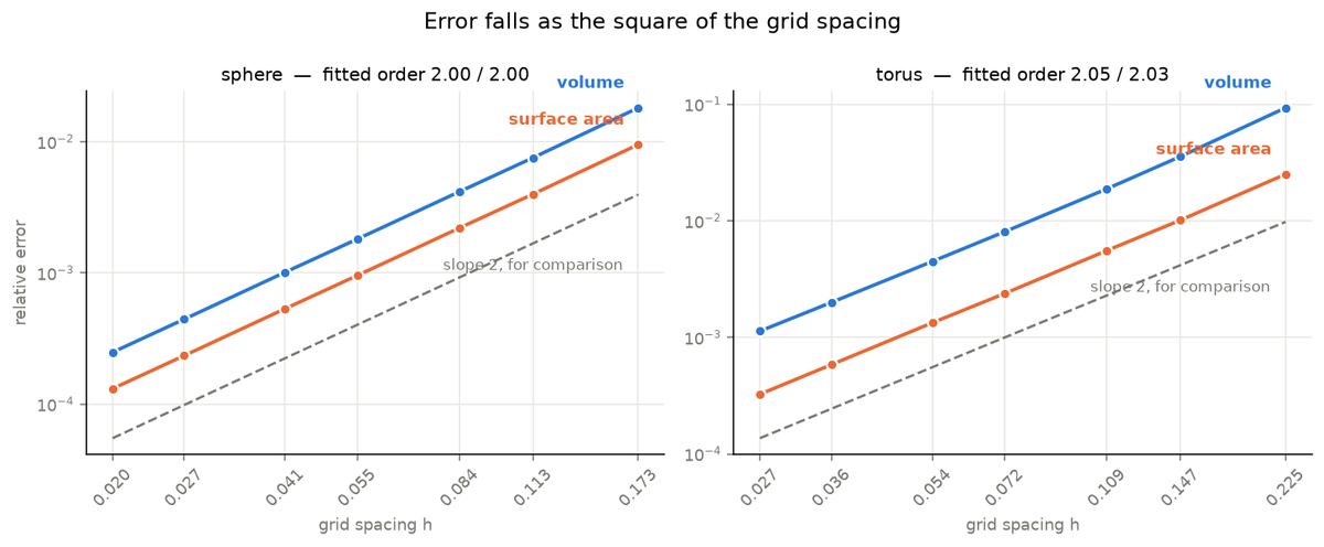
Marching cubes
The error is exactly second order, and that fixes the cost
Show the resultFitting
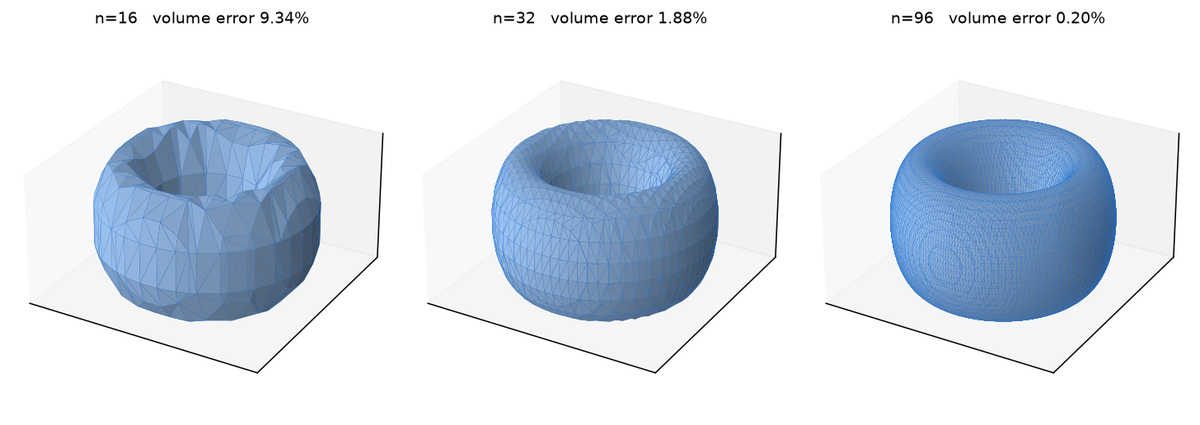
log(error)againstlog(h)gives the observed order of convergence:All six fits land within 0.05 of 2.00. Halving the grid spacing quarters the error — and costs eight times the memory and roughly six times the time. That is the whole trade, and it means accuracy here is bought at a known, unflattering rate: ten times the time buys about three times the accuracy, not ten.
Vertex distance converging at the same order as volume is the useful check. If the mesh were in the right place but the wrong size, the two would disagree.
ground truth closed form — sphere `4/3·π·r³`, `4·π·r²`; torus `2·π²·R·a²`, `4·π²·R·a` grids 16³ to 128³, seven resolutions variants `lewiner`, `lorensen` measurements volume error, area error, vertex distance to the true surface, time 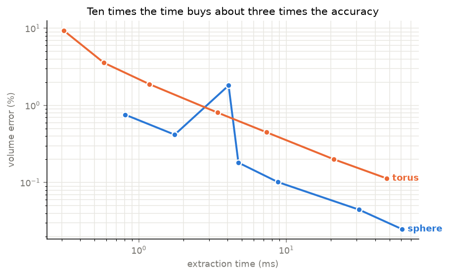
- 28.2354dB PSNR (test)
NeRF: mesh or novel view
Nearly all of the model is the lookup table, and it memorises
Show the resultThe MLP has 9,555 parameters. The hash table has 16.78 million — 1,756× more. So this is not a network that learned a scene so much as a lookup structure that stored one, with a tiny decoder on top.
The train/test gap shows what that costs: 33.592 dB on training views against 28.235 on held-out ones, a gap of 5.357 dB. Rendering from a pose it was fitted on is markedly easier than rendering from one it was not, which is exactly what a memorising representation predicts and what a single training-view render would have concealed.
The per-view spread matters as much as the mean. The worst held-out view scores 18.933 against a best of 34.242 — a range of 15.3 dB on the same trained model. A single averaged PSNR hides that some viewpoints are reconstructed far worse than others.
split PSNR test 28.2354 - Monocular depth
Monocular depth
The alignment protocol moves the score more than the model does
Show the resultDepth Anything V2 is a relative depth model — affine-invariant in disparity, meaning it recovers depth ordering up to an unknown scale and shift. The protocol most write-ups reach for, median-scaling in depth space, fits only the scale and leaves the shift unmodelled.
Both columns below score the same predictions:
δ Reported under the wrong protocol, this model looks roughly half as good as it is, and the number would read as a fact about the model rather than about the measurement.
The fitted disparity transform is reported rather than hidden, because it is the thing a single image cannot determine: scale 0.0848 (sd 0.03078), shift 0.25174 (sd 0.09518).
That shift standard deviation, 0.09518, happens to equal
abs_relto five decimals. It is a coincidence, not a copied field: the run computes and prints the fit statistics on a separate path from the metrics, and the log reports them independently.images 654 — the complete official NYU v2 test split ground truth measured depth, uint16 millimetres evaluation range 0.01–10.0 m, the NYU convention raw model output disparity — determined empirically, Spearman +0.9052 against ground-truth disparity (from the run log), not assumed 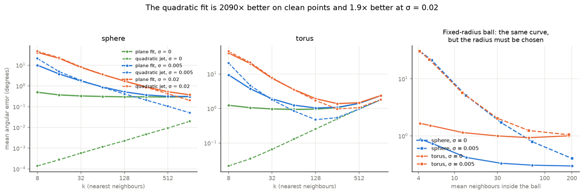
Normal estimation
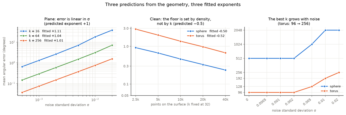
Three predictions from the geometry, three fitted exponents
Show the resultEach regime has an exponent that follows from the geometry rather than from the data, so the run either reproduces it or contradicts it.
surfaces plane (zero curvature), sphere (curvature 1.0), torus tube (curvature 2.857) ground truth analytic normals; error is the unsigned angle, so an unoriented PCA direction is scored fairly swept k from 4 to 2048, σ from 0 to 0.02, 2500 to 40000 points estimators PCA over k nearest · PCA over a fixed-radius ball · quadratic (jet) fit 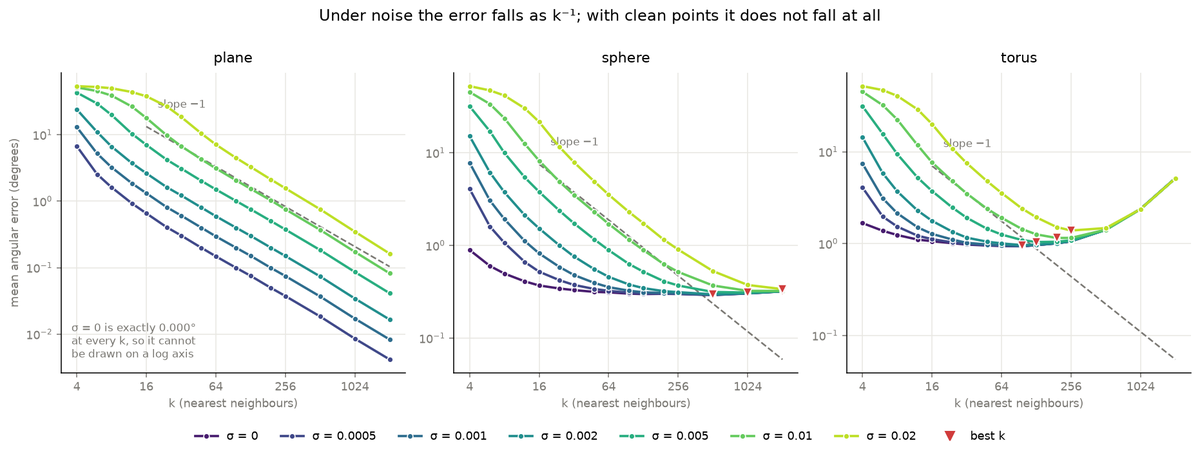
Point cloud decimation
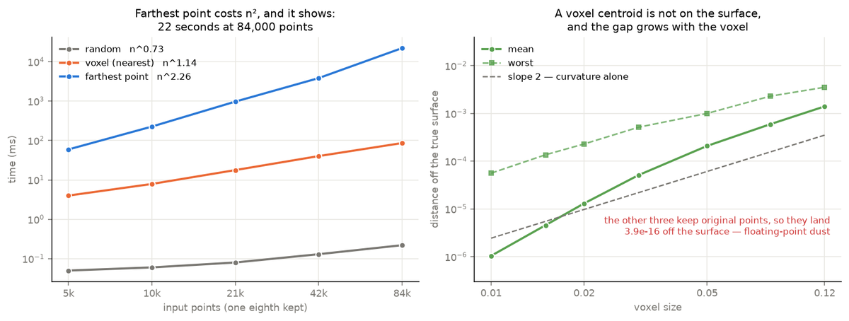
The metric usually quoted is the one that cannot tell these apart
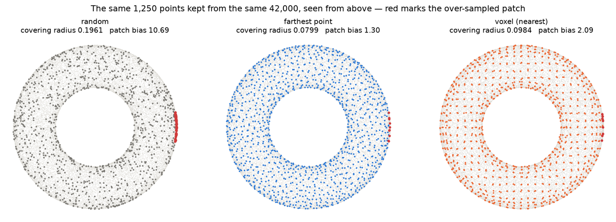
Show the resultChamfer distance back to the original cloud is what decimation is normally scored on. Across every matched count, the spread between the best and worst method on that metric is between 1.24× and 1.87×. On covering radius — the largest distance from any original point to its nearest kept point — the same four methods differ by up to 3.28×, and on density bias by nearly 10×.
Chamfer is a mean over every point, so a handful of badly served regions barely move it. The covering radius is the worst case, and the worst case is what decides whether a later surface fit, normal estimate or collision test has anything local to work with.
cloud 42000 points on a torus (R = 1, a = 0.35), of which 2222 lie in an over-sampled patch planted ground truth the patch's area is `a·2wu·(R·2wv + a(sin(v0+wv) − sin(v0−wv)))` = 0.08482102920624893, a 0.61% share of the surface; the input holds 5.2904761904761906% of its points there, a bias of 8.618248400757404 measured Chamfer back to the original, covering radius, distance off the true surface, density bias, wall clock retained 300 to 20000 points, matched across methods by bisecting the voxel size 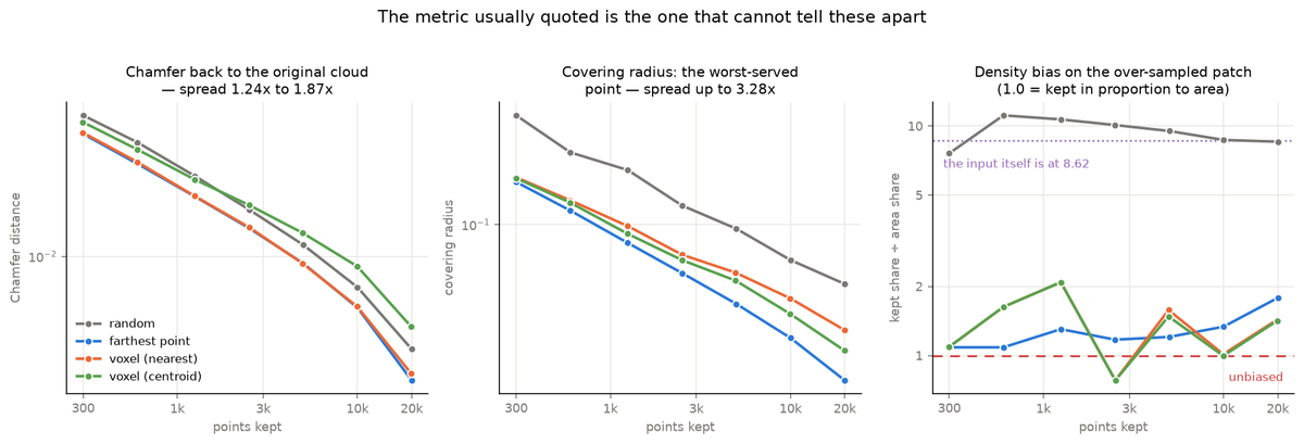
- 0.8254instance mIoU (test)
Point cloud segmentation
The two mIoUs disagree because rare categories are hard
Show the resultInstance mIoU averages over shapes, class mIoU averages over categories. They differ by 0.0552 on test, and the reason is visible once categories are split by how many test shapes they have:
A gap of 0.1233. Class mIoU weights a category with 12 shapes the same as one with 704, so it reports the rare-category difficulty that instance mIoU averages away.
Worst and best on test:
Laptop at 0.9547 with only 83 shapes shows the driver is not sample count alone — a laptop is two near-planar parts with an unambiguous boundary, while a rocket's fins, body and nose meet at boundaries that are genuinely ambiguous. Sample size and intrinsic difficulty both contribute, and this experiment does not separate them.
split instance mIoU train 0.8583 val 0.8516 test 0.8254 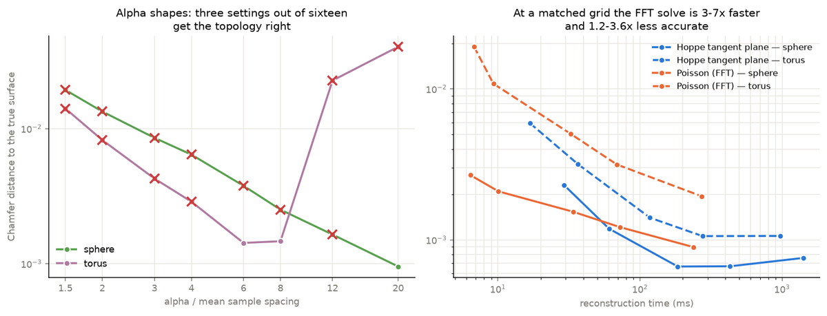
Surface reconstruction
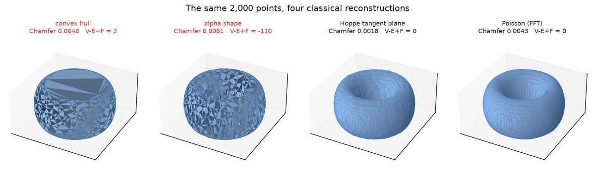
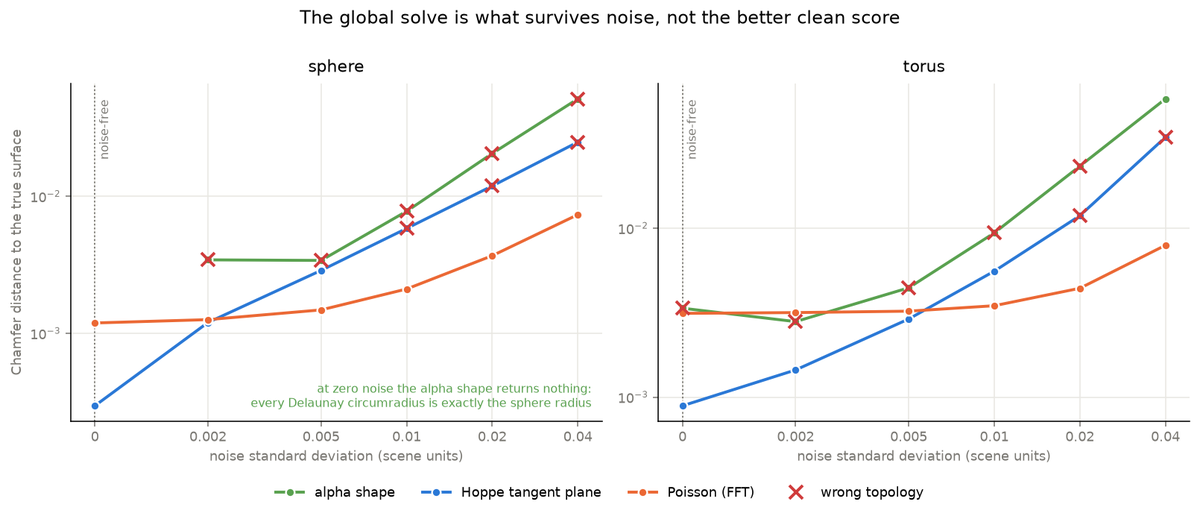
The convex hull is the most accurate method on the sphere and the only one that cannot be fixed on the torus
Show the resultOn a convex surface the hull converges as
n^−1.00— faster than every other method tested, and at 8000 points it is the most accurate of the four (0.00052) while taking 18.1 ms against Hoppe's 782.1 ms.On the torus the same method is stuck at 0.065 and sixteen times more points change it by −4.7%: the fitted exponent is −0.02, which is a flat line with measurement noise on it. Its Euler characteristic is 2 at every size, because a hull has no way to represent a hole. This is the clean case of a method that is not slowly wrong but structurally wrong, and the exponent is how you tell the two apart without looking at a picture.
surfaces unit sphere, torus (R = 1, a = 0.35) ground truth ` methods convex hull · alpha shape (3-D Delaunay) · Hoppe tangent plane · Poisson (FFT) varied 500–8000 points, noise σ = 0 to 0.04, alpha, grid resolution normals estimated by PCA and oriented by spanning-tree propagation — not given 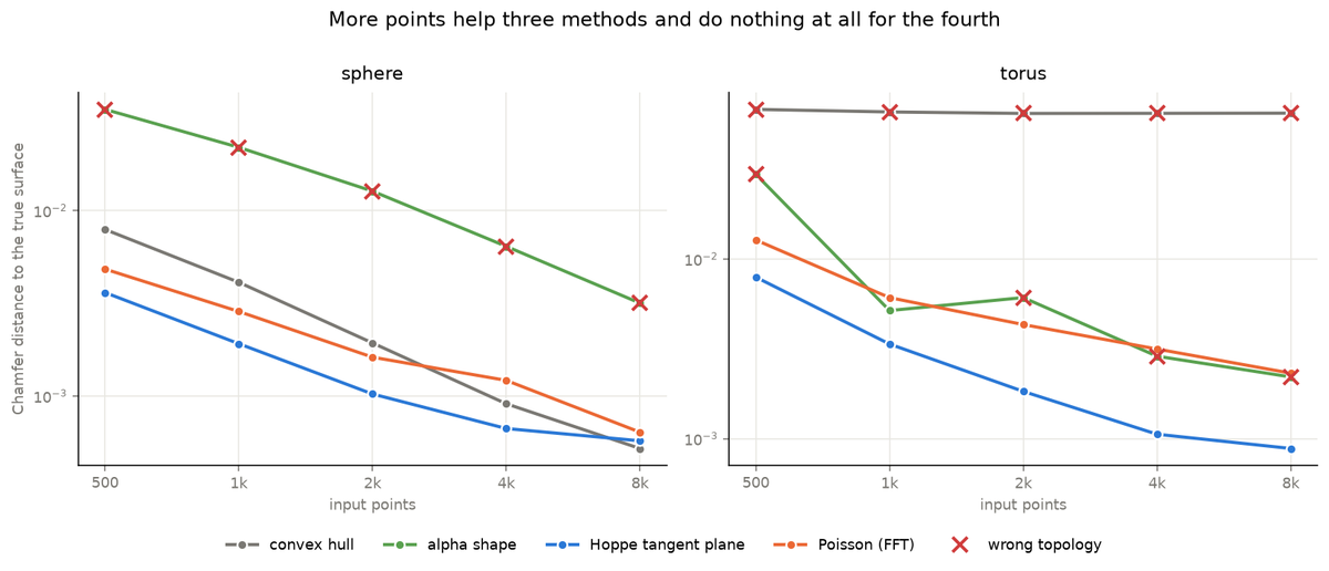
Two-view triangulation
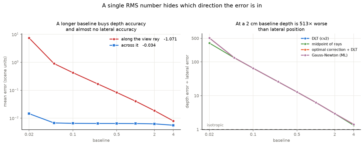
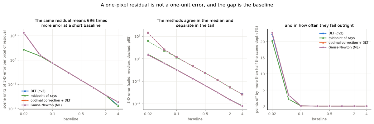
Two predictions from the geometry, two fitted exponents
Show the resultBoth hold to within 1.2%. The baseline fit uses baselines of 0.1 and above: below that the error is a sizeable fraction of the scene depth, points start landing behind the camera and the error saturates instead of growing, so a fit across that boundary would be measuring the saturation.
cameras 1280 × 960, focal length 1000 px, second camera verged on the scene centre scene 2000 points at depths 4.0 to 8.0, mean depth 6 ground truth the 3-D points themselves; only the pixel measurements are perturbed methods `cv2.triangulatePoints` (DLT) · midpoint of rays · `cv2.correctMatches` + DLT · Gauss-Newton on reprojection error (the ML estimate) swept pixel noise σ = 0 to 10 px, baseline 0.02 to 4.0 scene units 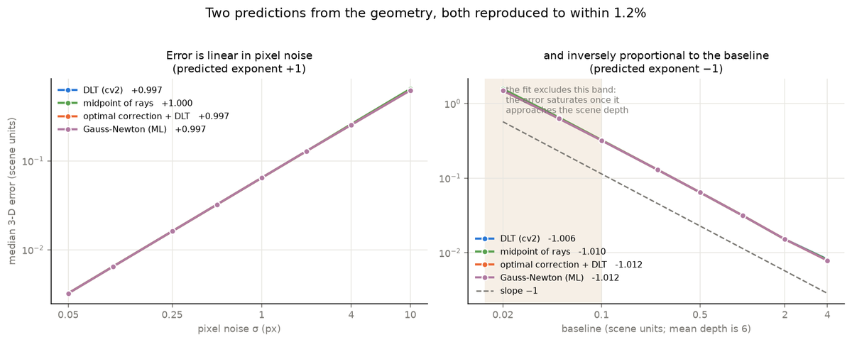
- Volumetric segmentation
Volumetric segmentation
The headline metric is blind to the failure that matters
Show the resultBraTS 2020 is 368 multi-modal brain MRI volumes with three annotated tumour subregions.
On 6 of the 55 test patients the enhancing-tumour Dice is exactly 0.0000 — the model and the annotation share no enhancing voxel at all. The whole-tumour score does not notice:
Whole tumour falls by 0.02. Tumour core falls by 0.40. Five of those six patients still clear the 0.80 whole-tumour bar.
Case 361 is the clearest: a whole-tumour Dice of 0.8735, above the bar, with a tumour core of 0.0322. Whole tumour is the union of all three labels, and that union is dominated by peritumoural oedema — the largest and most separable region. A model can own the oedema and miss the enhancing rim entirely while the headline barely moves.
Had this project reported one number, it would have reported 0.8734 and been wrong about what the model does.
split patients train 258 val 55 test 55
Recognition, Pose, Video & Anomaly
Open the page →Networks that find things: defects, people, actions and the unusual. Each scored on a held-out split against a bar set from published results beforehand.
- 0.7633frame AUC
Anomaly detection
AUC says it works, the operating points say it cannot be used
Show the resultAnomalous frames are 7.666% of the test set. At the operating point that catches 80% of them, 43.754% of all frames are flagged — so the overwhelming majority of alarms are on normal footage, and raising recall to 0.90035 pushes false positives past half of everything.
A single AUC of 0.76329 reads as a working system. It is the same model at every threshold, and there is no threshold at which it is usable. That gap is the entire reason this write-up leads with the caveat rather than the metric: AUC is a ranking summary over a pooled frame set, and pooled ranking quality is not operational performance.
features frozen ImageNet ResNet-50 (`IMAGENET1K_V2`), 2048-d, nothing fine-tuned supervision at train video-level only — "this video contains an anomaly" labels at test official per-frame temporal annotations, fetched at run time annotation coverage every official test video matched an annotation, and the folder label agreed with the annotation on every one of them (from the run log) train / test videos 1582 / 283, zero video-name overlap test frames scored 111134, of which 8520 anomalous (7.666%) frame size 64 × 64 — this dataset copy is decimated and small 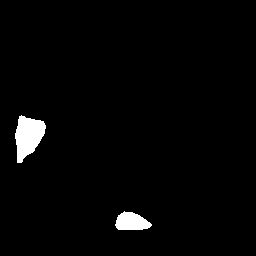
Defect localisation
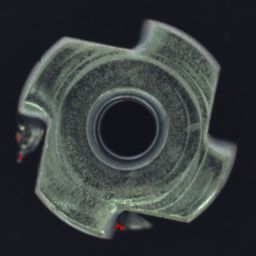
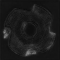
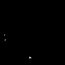
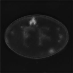
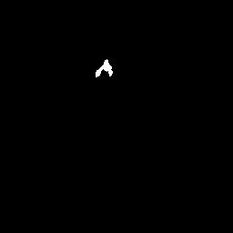
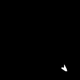
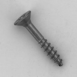
Trained from scratch for 120 epochs across 12 MVTec AD object categories
0.9583 pixel AP (test)Show the resultPixel-level localisation of manufacturing defects.
- Trained from scratch for 120 epochs across 12 MVTec AD object categories.
- Test pixel AP 0.9583, pooled IoU 0.8033, per-image IoU 0.6232. The decision threshold was tuned on the validation split.
split pixel AP train 0.9839 val 0.9565 test 0.9583 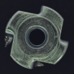

- 0.9379mean AUROC
Industrial anomaly
What the features are worth depends on what you are inspecting
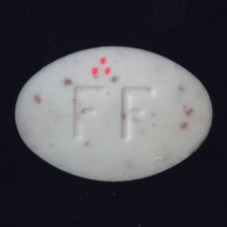
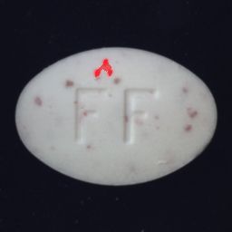
Show the resultThe raw-pixel control runs the same bank, the same distance and the same scoring rule — only the representation differs. Splitting the fifteen categories into MVTec's own texture and object groups:
The representation is worth 2.3× more on objects than on textures. On a texture, a defect is a local statistical break and raw pixels already catch most of it —
leatherscores 0.9808 on pixels alone against 1.0000 with features. On an object, the defect is a part being wrong in a specific place, and raw pixels are near chance:metal_nutscores 0.4040 on pixels — below 0.5, so worse than guessing — against 0.9878 with features.Without the control, 0.9379 would have read as a fact about the method. It is mostly a fact about where the representation is doing the work.
mean image AUROC frozen ResNet-50 features 0.9379 raw 32×32 pixels, identical pipeline 0.6700 published PatchCore (trains a coreset) ~0.991 - 0.656OKS AP
Pose estimation
The per-joint ranking inverts with tolerance
Show the resultTwo different joints are "the worst" depending only on the threshold:
- At PCK@0.2 the ankles are last (0.918, 0.9192) and the hips sit comfortably mid-table (0.9418, 0.9438). - At PCK@0.05 the hips are last by a distance (0.6388, 0.6389), while the ankles (0.745, 0.7496) rank above the knees and below the wrists.
The median-error column explains why, and the two failure modes are genuinely different:
- Hips carry large typical error but a light tail. Median error 0.03637 is the worst on the body, against 0.00783 at the eyes. Yet its PCK@0.2 is 0.9418, so few hip predictions miss by more than that tolerance. A hip has no visible landmark; it is an interior anatomical guess, so almost every prediction is a little bit off and almost none is wildly off. - Ankles carry small typical error but a heavy tail. Median error 0.02244 is well under the hips', yet its PCK@0.2 of 0.918 is the lowest on the body — the heaviest tail there is. An ankle is a sharp, visible landmark that is either found precisely or lost completely to occlusion and motion blur.
So "wrists and ankles are worst" describes a tail, and the hips' problem is a bias. A single PCK number cannot distinguish those, and the one most often quoted — the loose one — reports only the tail.
### The loose threshold also hides almost all per-joint structure
At PCK@0.2 every joint scores between 0.918 and 0.9838. The table is nearly flat and reads as "this model is uniformly good". The same predictions at PCK@0.05 run from 0.6388 to 0.9607 and rank the joints in a different order. The per-joint table is only informative at a tolerance tight enough to resolve it.
Grouped at PCK@0.2, extremities (wrists + ankles, 13698 joints) score 0.92524 against 0.95931 for the core (shoulders + hips + nose, 24477 joints) — a real but modest gap that understates what is happening underneath.
images scored 2346 — every image this dataset copy ships that has an annotated person ground-truth persons 6352, of which 6237 matched a detection at box IoU ≥ 0.5 labelled joints scored 67391 of 68215 protocol official COCO OKS AP via `pycocotools`, plus PCK at three tolerances 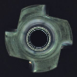
Product matting
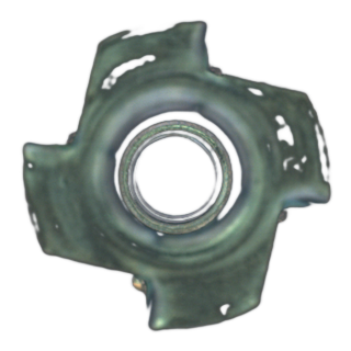
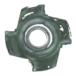
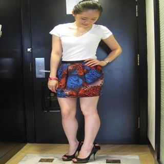
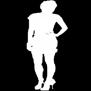
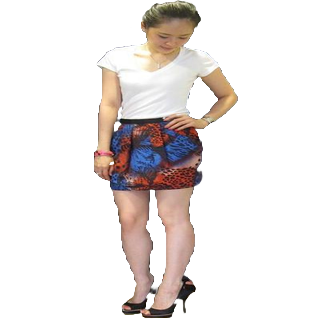
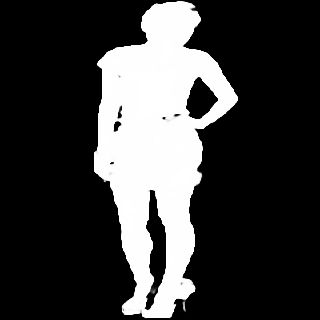
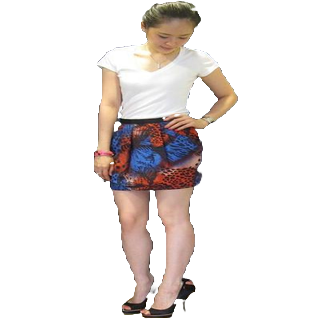
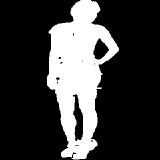
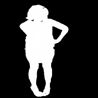
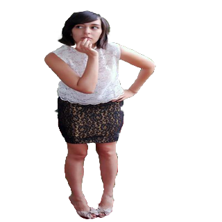
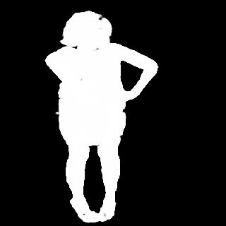
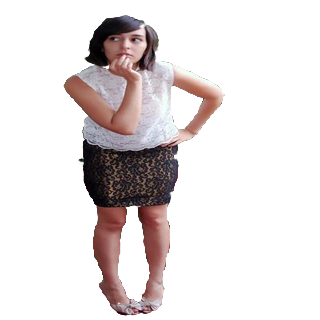
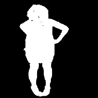
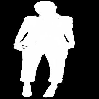
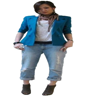
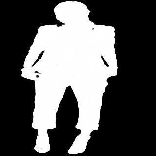
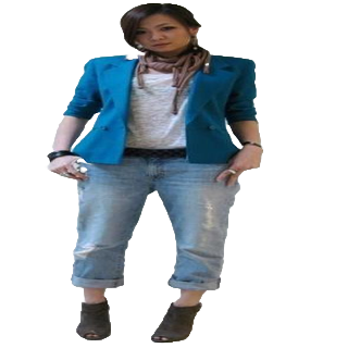
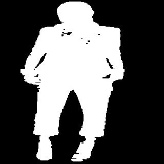
U2-Net fine-tuned for 100 epochs with BCE plus soft-dice at 320x320
0.9611 IoU (test)Show the resultAlpha matte extraction for background removal.
- U2-Net fine-tuned for 100 epochs with BCE plus soft-dice at 320x320.
- Ground-truth mattes are derived by Otsu thresholding with hole filling.
split IoU train 0.9903 val 0.9625 test 0.9611 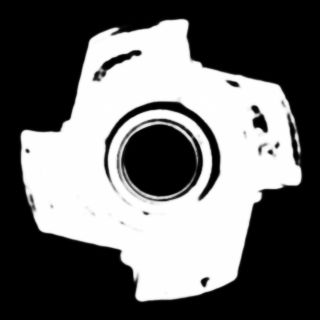




- 0.8094top-1 (held out test)
Video action recognition
The confusion pairs are all within-domain
Show the resultNot one of these is a random mistake. Read as pairs they are almost tautological:
- Same sport, different act — CricketShot/CricketBowling, BoxingPunchingBag/BoxingSpeedBag, BalanceBeam/ParallelBars, HammerThrow/ThrowDiscus. - Same medium — FrontCrawl/BreastStroke (a pool), Kayaking/Rafting (a river). - Same instrument family — PlayingDhol/PlayingTabla (drums), PlayingFlute/PlayingViolin. - Same scene and posture — BrushingTeeth confused with both ShavingBeard and ApplyLipstick: a hand raised to the face at a bathroom mirror, three times over. - Same object kinematics — YoYo/Nunchucks, two things swung on a string.
The pattern says what the representation is doing. Kinetics features encode scene, object and context strongly, and a linear read-out of them separates contexts almost perfectly — top-5 is 0.96405, so the right answer is nearly always among the handful of candidates. What a linear probe cannot do is the fine-grained temporal discrimination within a context: which swimming stroke, which cricket action, which bathroom gesture.
That is also why the worst classes are what they are:
Every one of them has a near-twin elsewhere in the label set. The gap between top-1 0.80941 and top-5 0.96405 is almost entirely this: the model is choosing wrongly among a small set of correct-context neighbours.
split official UCF101 split 1 (`trainlist01`/`testlist01`), fetched at run time and validated against the published split-1 list sizes before use classes 101 videos used 5050 train / 1082 val / 3783 test leakage checks file overlap 0 and clip-group overlap 0 on all three split pairs decode success 1.0 on all three splits device cpu — the Kaggle weekly GPU quota was exhausted - Video instance segmentation
Video instance segmentation
The model's video problem is association, not segmentation
Show the resultThe two temporal numbers disagree, and the disagreement is the result.
Frame-to-frame mask IoU for the predictions is 0.78932. For the ground-truth masks of the same objects over the same frame pairs it is 0.78441. The gap is −0.00491 — predicted masks change very slightly less between consecutive frames than the true masks do. By that measure the output is not jittery at all.
Yet on 0.10342 of consecutive frame pairs where the object is detected in both frames, the mask covering it is not linked to the mask that covered it a frame earlier. The shape is stable; the correspondence is what breaks.
This is exactly why the GT baseline has to be measured alongside. Reporting predicted frame-to-frame IoU alone (0.78932) would read as "temporally consistent". Reporting the jump rate alone would read as "jittery masks". Neither is true, and the fix each would suggest is different: what this needs is a tracking component, not a smoother mask head.
The GT number is also what makes the predicted one interpretable. Without it, 0.78932 could mean a stable model or a slow-moving dataset — DAVIS objects move enough that the true masks overlap themselves by only 0.78441 between frames.
split official `ImageSets/2017/val.txt` — 30 sequences frames scored 1999 ground-truth objects 61, across 3929 instance-frames predicted masks 17632 model COCO-pretrained, never trained on DAVIS; published COCO mask AP 34.6
Generation & Restoration
Open the page →Image-to-image restoration and translation, plus generation from text. Every project ships the images it produced alongside the number it scored.
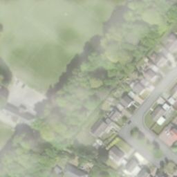
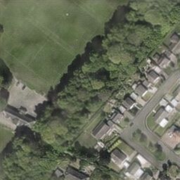
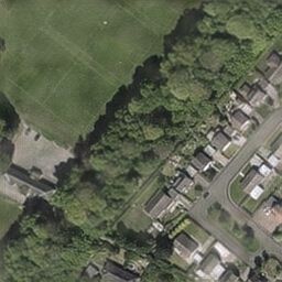
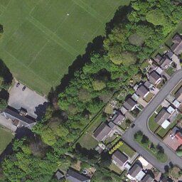
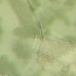
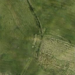
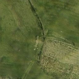
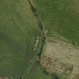
Cloud removal
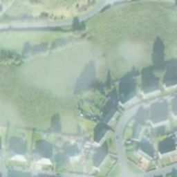
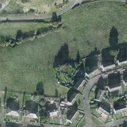
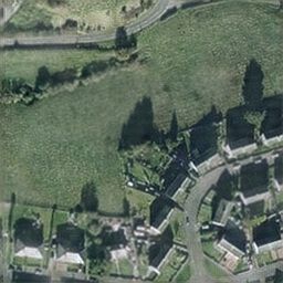
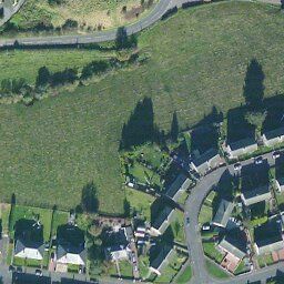
Fine-tuned from the published RICE2 generator for 60 epochs on 1,600 training pairs
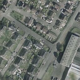
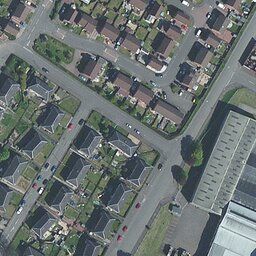
23.6964 dB PSNR (test)Show the resultRemove haze and cloud from aerial imagery.
- Fine-tuned from the published RICE2 generator for 60 epochs on 1,600 training pairs.
- Train 24.13 / val 23.97 / test 23.70 - a tight spread across all three splits.
split PSNR train n=1600 24.1264 val n=300 23.9666 test n=100 23.6964 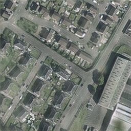

Colourisation
Trained from scratch for 100 epochs on 2,280 images, predicting the ab channels from L in Lab space
21.9107 dB PSNR (test)Show the resultPredict colour (ab) from luminance (L) in Lab space.
- Trained from scratch for 100 epochs on 2,280 images, predicting the ab channels from L in Lab space.
- The dataset was filtered for colour content: near-grey and low-saturation images were dropped when it was built.
split PSNR train n=428 22.5389 val n=428 22.2671 test n=142 21.9107 




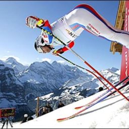
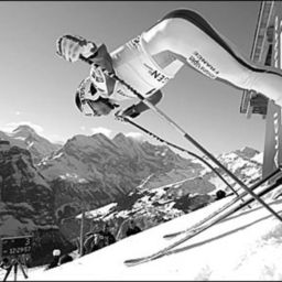
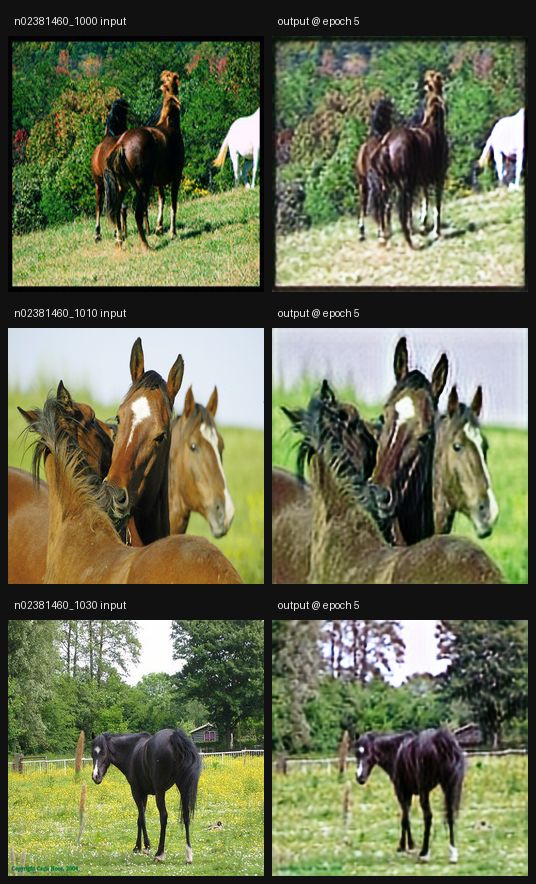
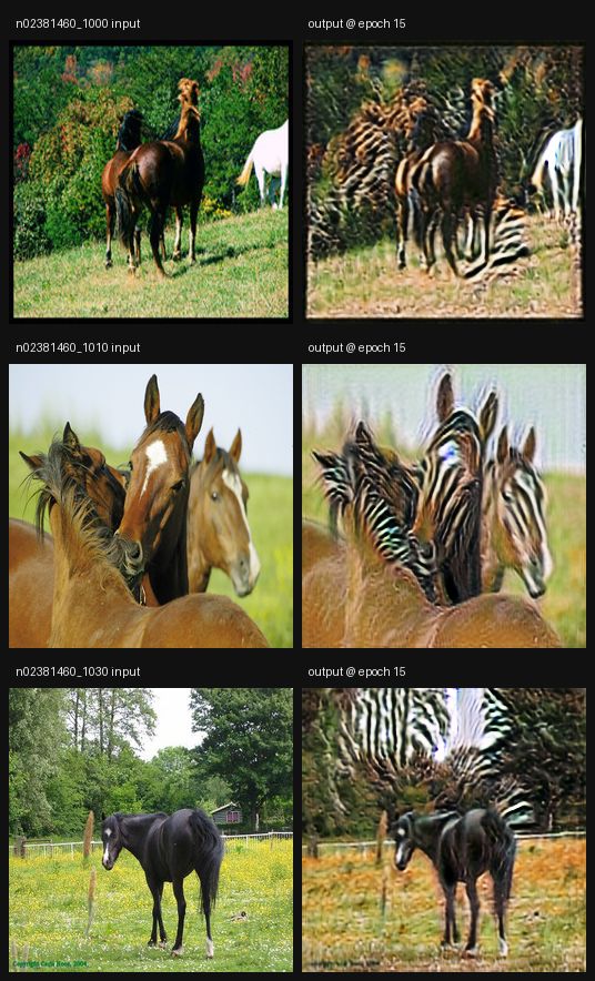
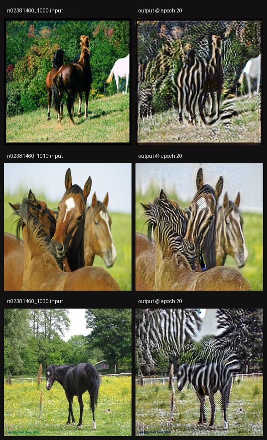
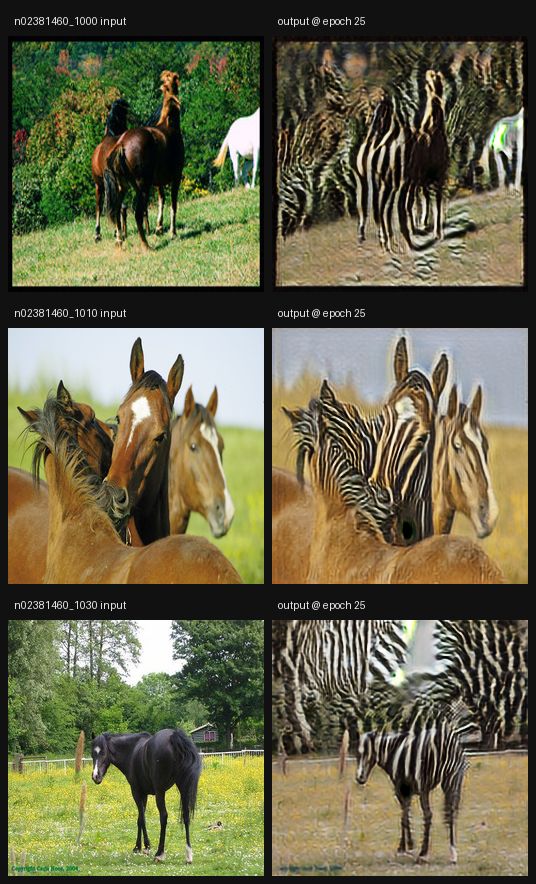
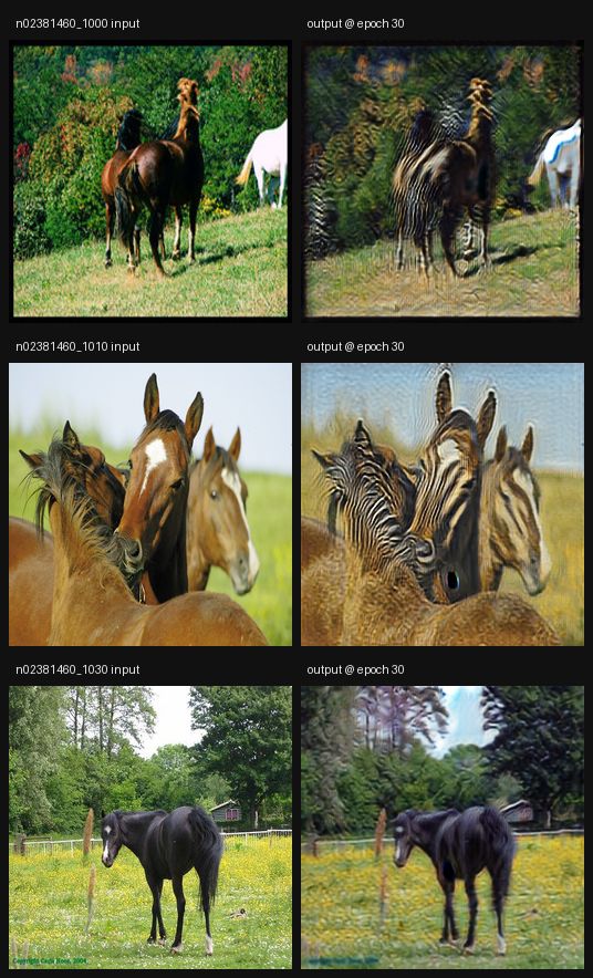
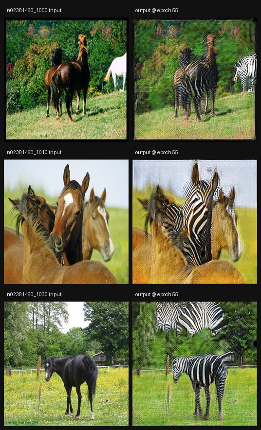
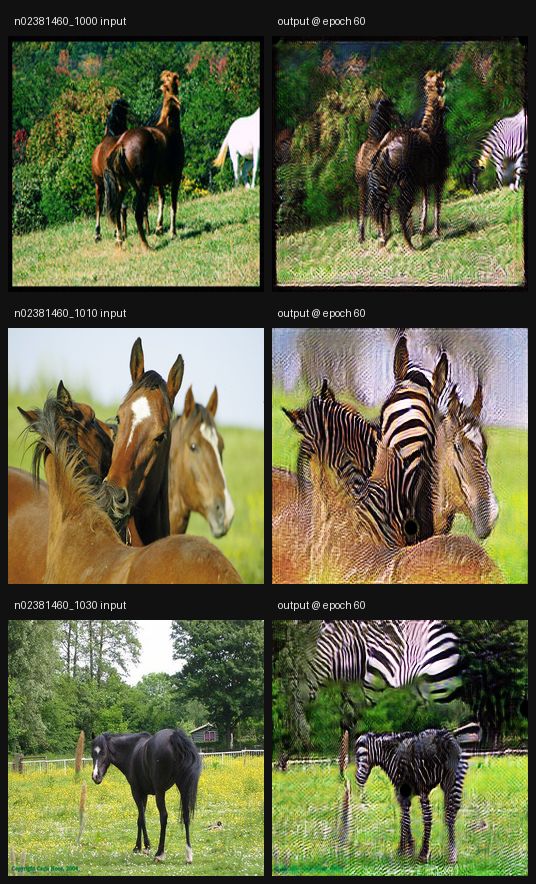
CUT: horse to zebra
100 epochs on the horse2zebra set
Show the result- 100 epochs on the horse2zebra set. CUT is unpaired, so the result is shown as images rather than a pixel metric.
- Budget matched to cyclegan-h2z, which trains on the same data.
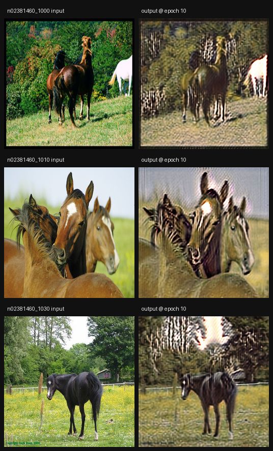
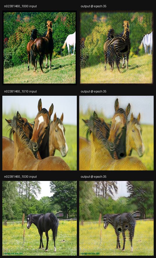
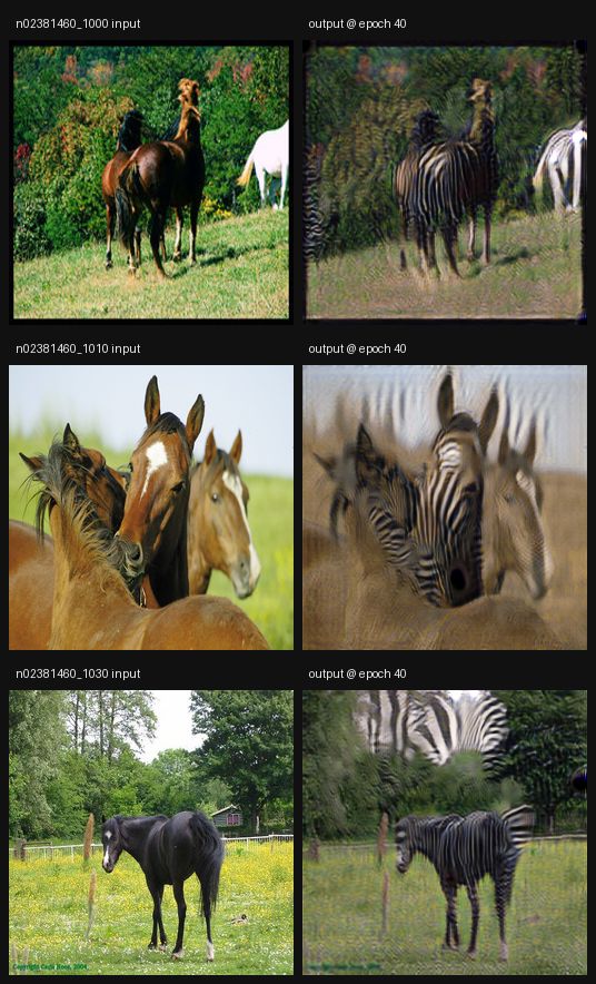
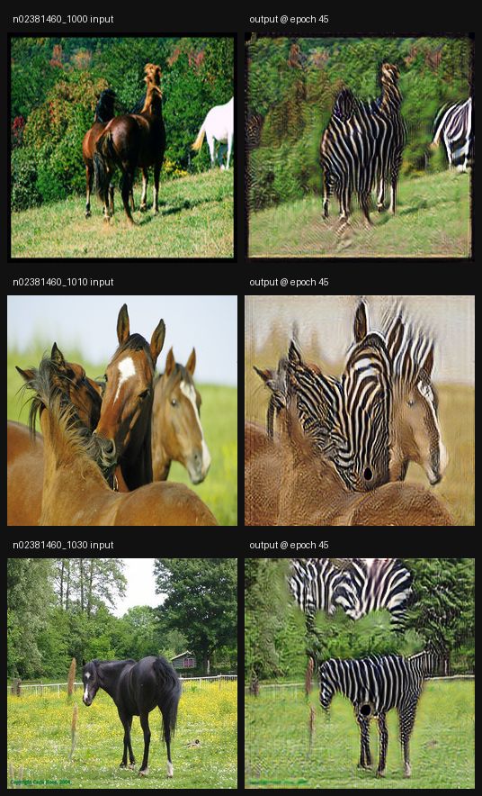
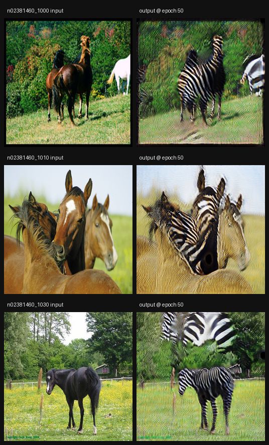
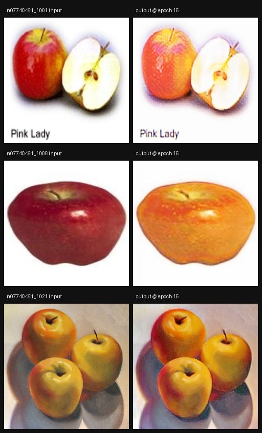
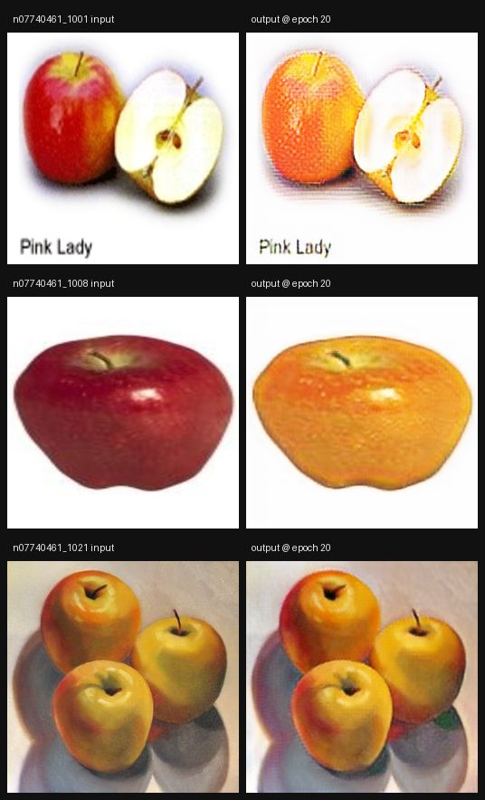
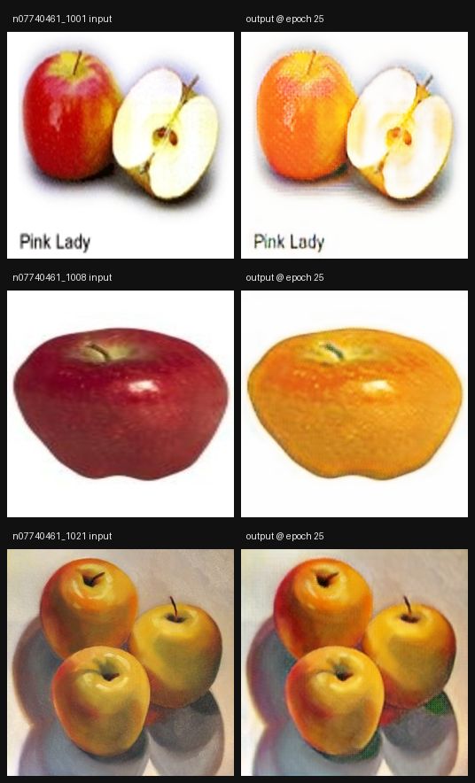
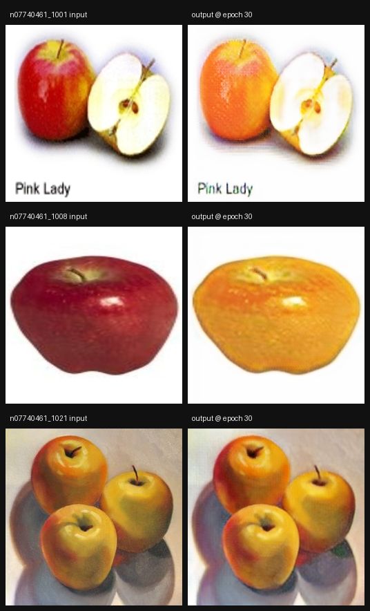
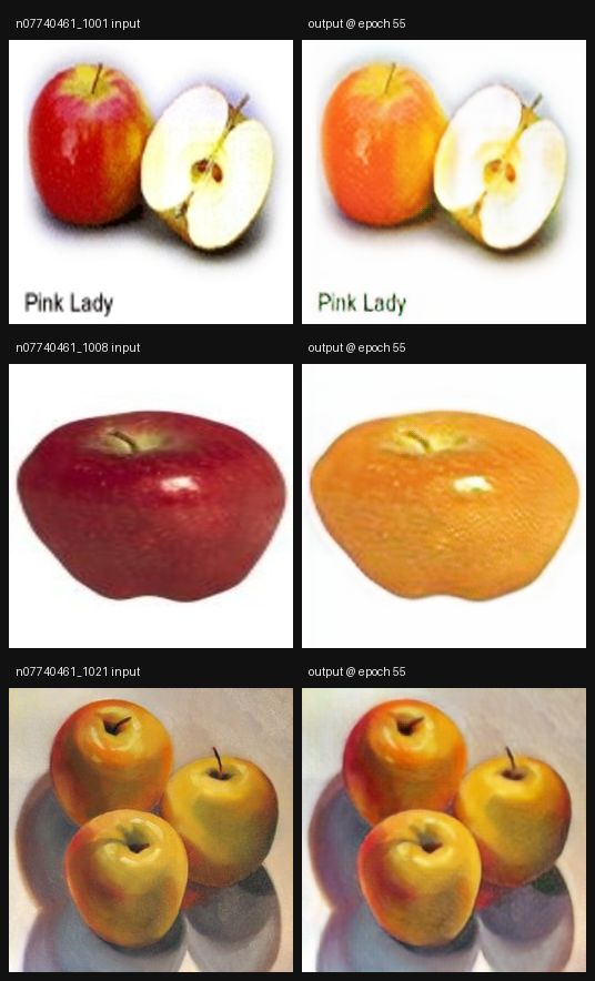
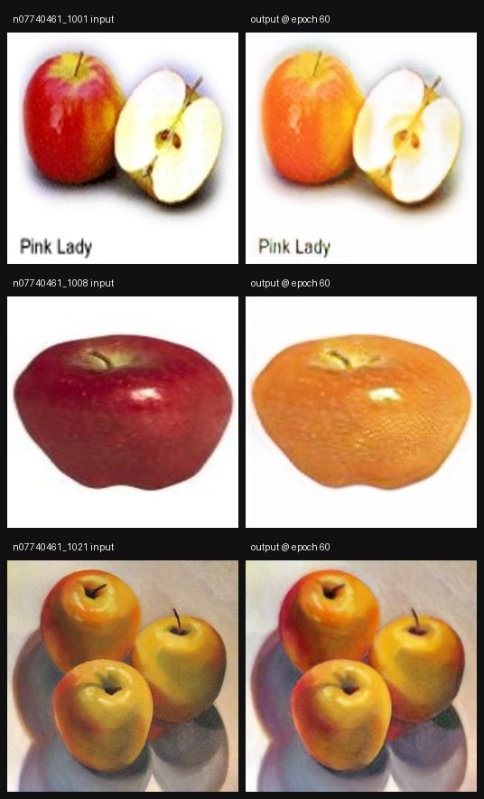
CycleGAN: apple to orange
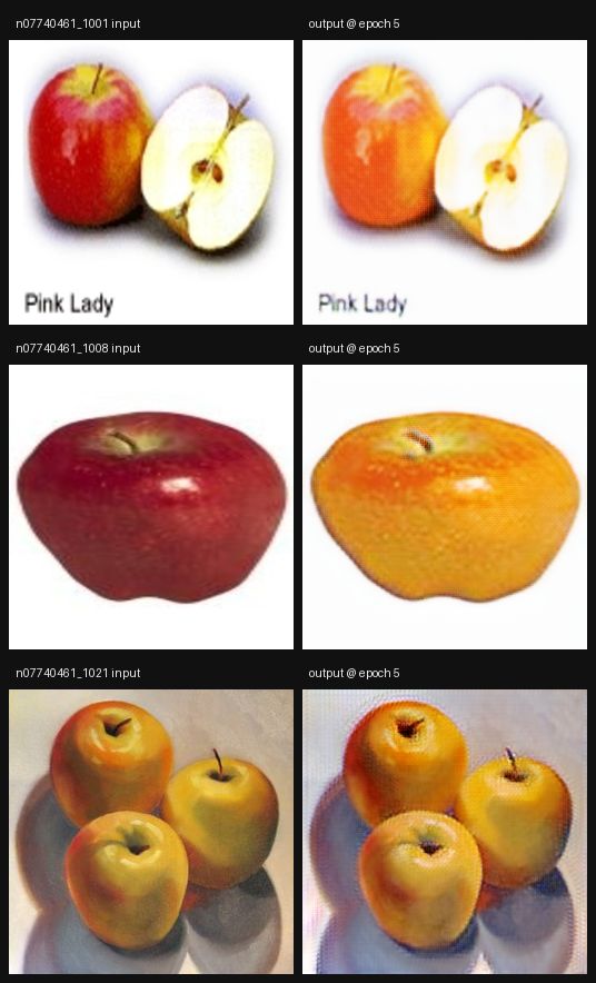
100 epochs on the apple2orange set, 50 at the base rate then 50 linearly decayed - the published schedule
-0.0958 negative cycle-consistency L1 on held-out images (val)Show the result- 100 epochs on the apple2orange set, 50 at the base rate then 50 linearly decayed - the published schedule.
- Samples show the same inputs translated at epochs 5 through 100.
split PSNR val n=60 -0.0958 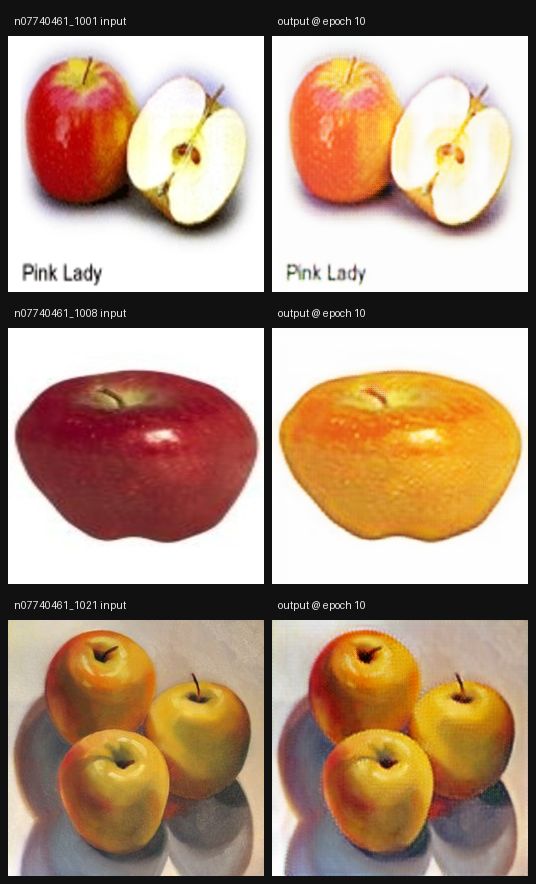
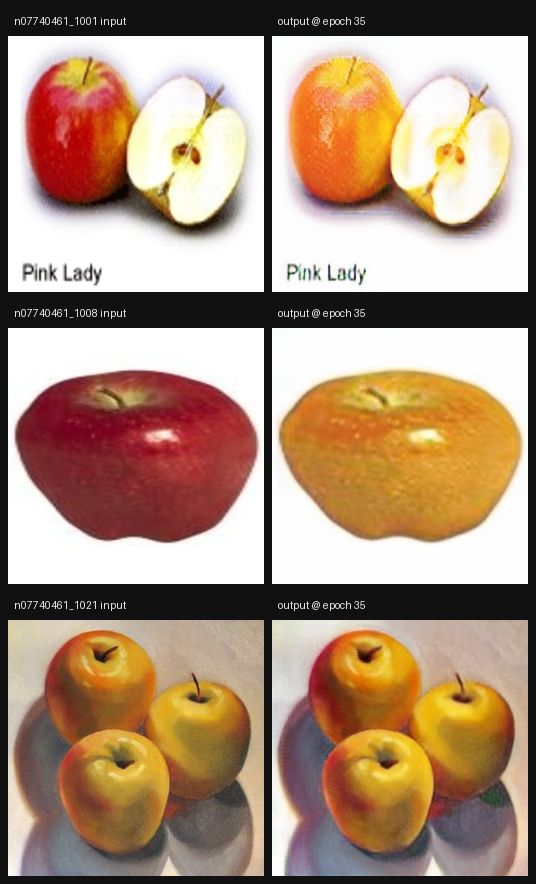
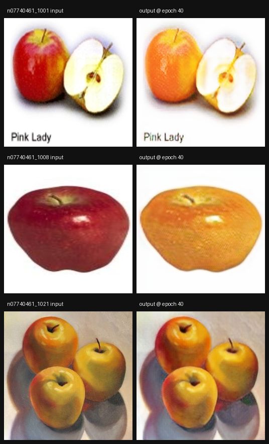
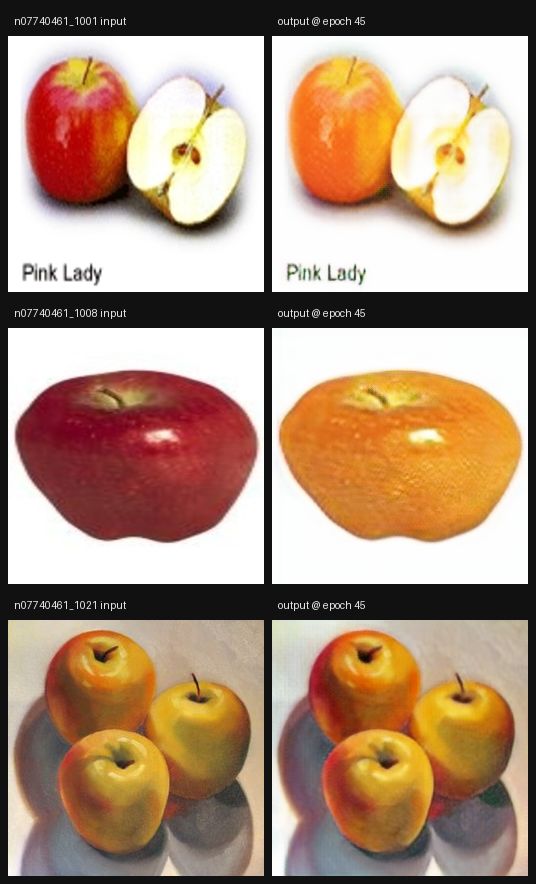
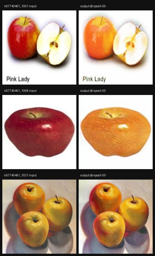
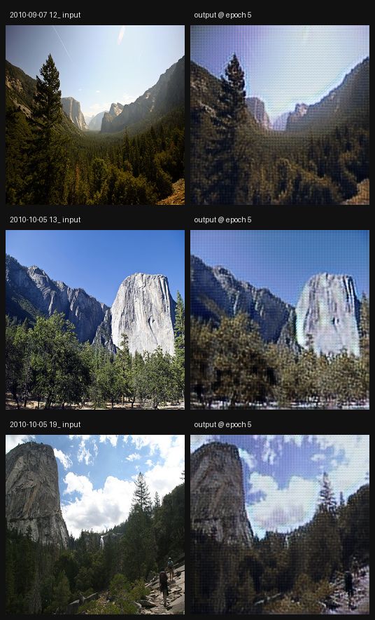
CycleGAN: summer to winter
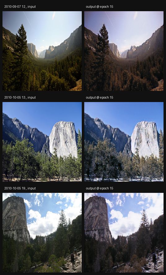
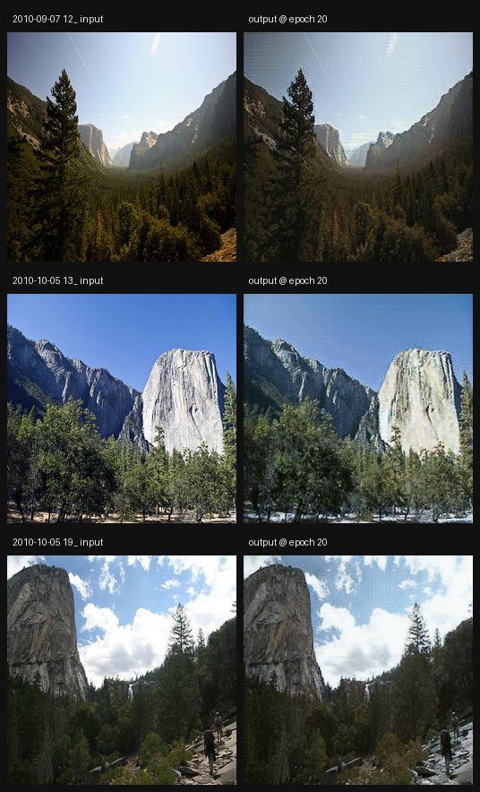
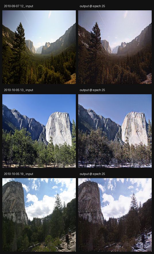
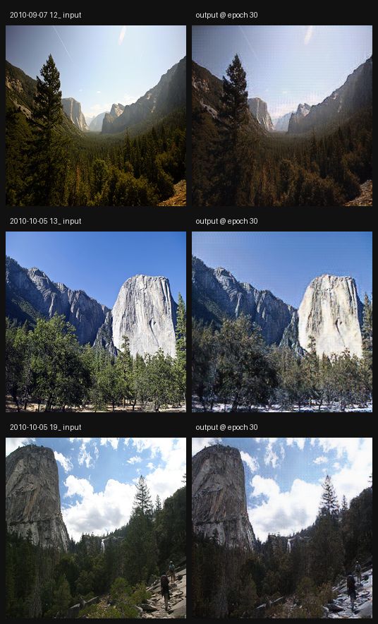
30 epochs on the summer2winter_yosemite set, not the 100 the other CycleGAN runs used
-0.1049 negative cycle-consistency L1 on held-out images (val)Show the result- 30 epochs on the summer2winter_yosemite set, not the 100 the other CycleGAN runs used. The run was stopped early: the GPU dropped to half its clock (1035 of 2100 MHz, 46 of 110 W) and an epoch went from 7 to 29 minutes, which put the remaining 70 epochs at about 34 hours for a cycle-consistency gain of 0.009 per 10 epochs.
- Samples show the same inputs translated at epochs 5 through 30, so the trend over training is visible even though the budget is shorter than apple2orange's.
split PSNR val n=60 -0.1049 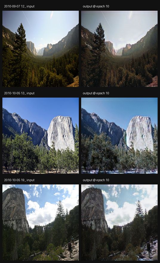
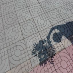
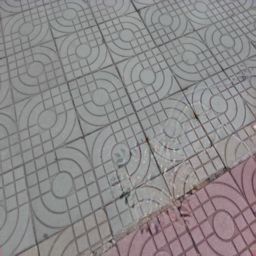
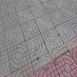
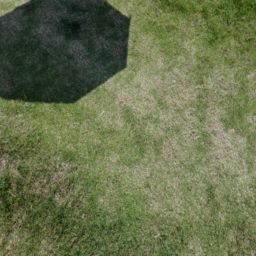
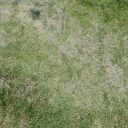
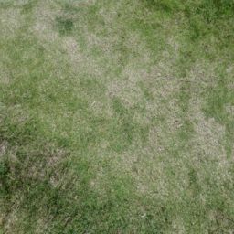
Document shadow removal
Fine-tuned for 56 epochs on 800 training pairs; the best val score came at epoch 50 and five further epochs did not beat it, so the run was stopped there
30.5951 dB PSNR (test)Show the resultRemove shadows cast across a photographed document page.
- Fine-tuned for 56 epochs on 800 training pairs; the best val score came at epoch 50 and five further epochs did not beat it, so the run was stopped there.
- Train 30.67 / val 30.49 / test 30.60 - a tight spread across all three splits.
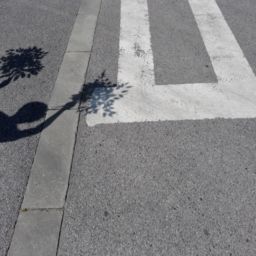
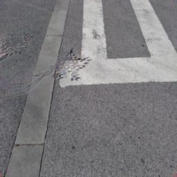
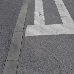
- Samples show the shadowed input, the published weights' output, this run's output and the ground truth.
split PSNR train n=800 30.6673 val n=150 30.4923 test n=50 30.5951 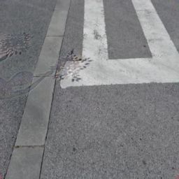




ESRGAN super-resolution
Trained with L1 + adversarial
28.6938 dB PSNR (test)Show the result- Trained with L1 + adversarial.
- Fine-tuned from the published x4 checkpoint into an x6 architecture, with the upsampling stage rebuilt for a factor of 6.
- 20,000 steps on 720 training frames, evaluated on held-out val and test splits.
split PSNR train n=720 28.3642 val n=135 27.8051 test n=45 28.6938 











Face restoration
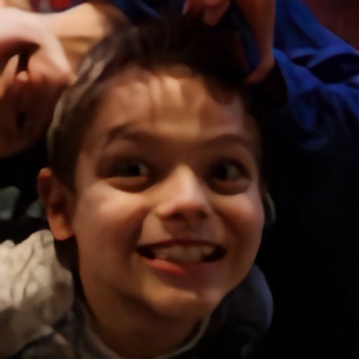
Generator fine-tuned with L1 on synthetically degraded FFHQ crops, 15,000 steps at batch 2
30.0195 dB PSNR (test)Show the resultRestore degraded face crops. Degradation is synthesised at load time.
- Generator fine-tuned with L1 on synthetically degraded FFHQ crops, 15,000 steps at batch 2.
- Sample images show the degraded input, the pretrained output and the fine-tuned output against ground truth.
split PSNR train n=150 30.0851 val n=150 29.9772 test n=50 30.0195 








MSRGAN super-resolution
Trained with L1 + adversarial
28.47 dB PSNR (test)Show the result- Trained with L1 + adversarial.
- Fine-tuned from the published x4 checkpoint into an x6 architecture, with the upsampling stage rebuilt for a factor of 6.
- 20,000 steps on 720 training frames, evaluated on held-out val and test splits.
split PSNR train n=720 28.1670 val n=135 27.5742 test n=45 28.4700 










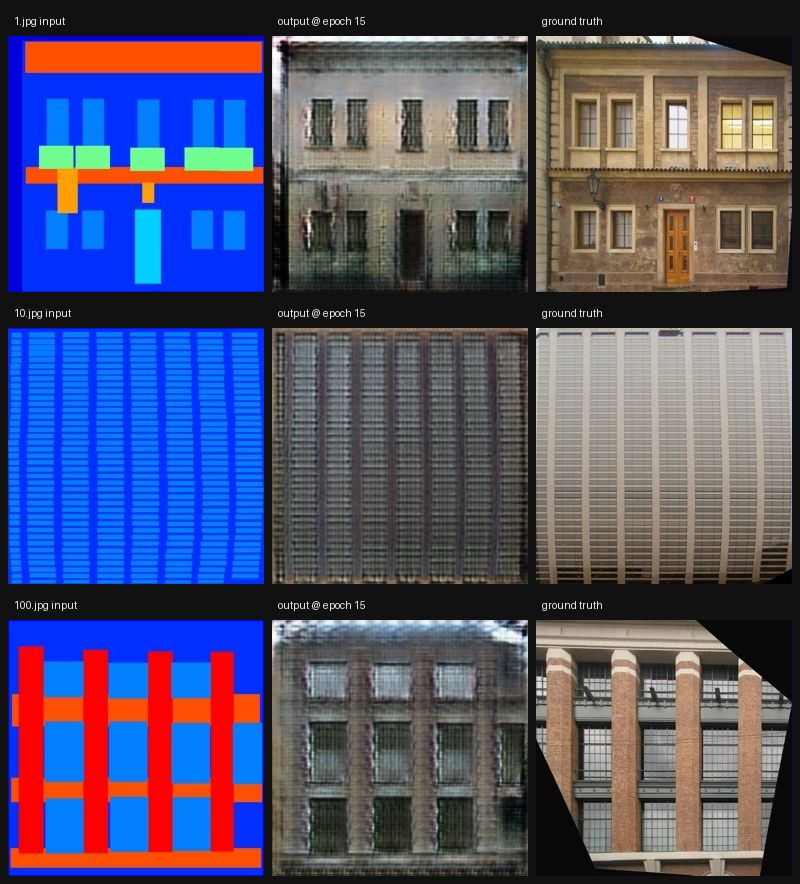
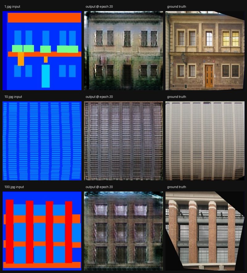
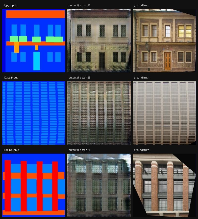
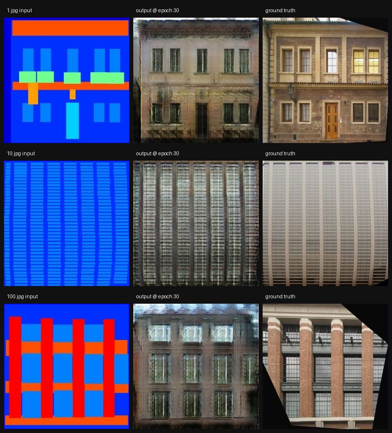
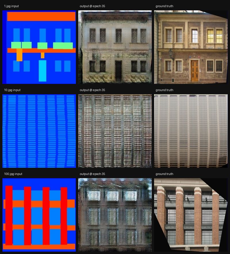
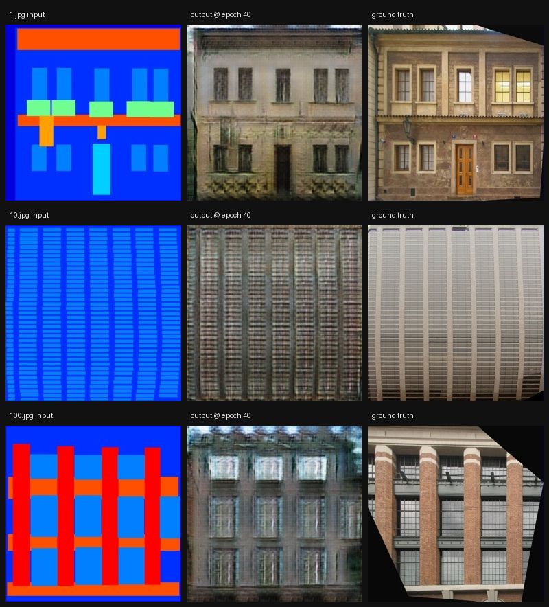
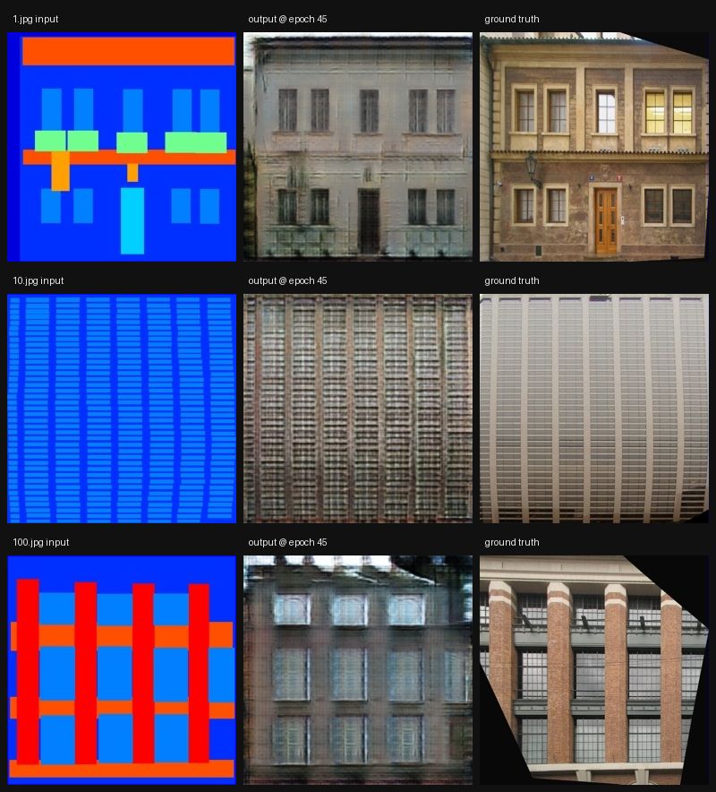
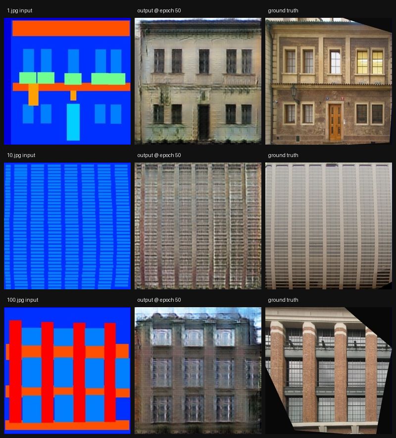
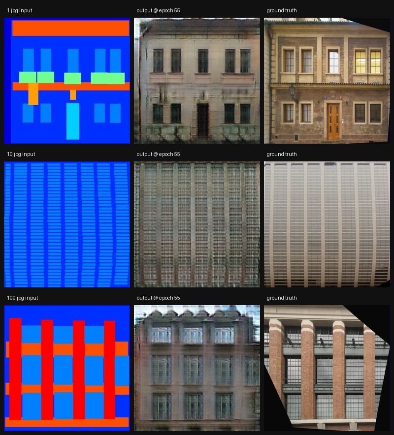
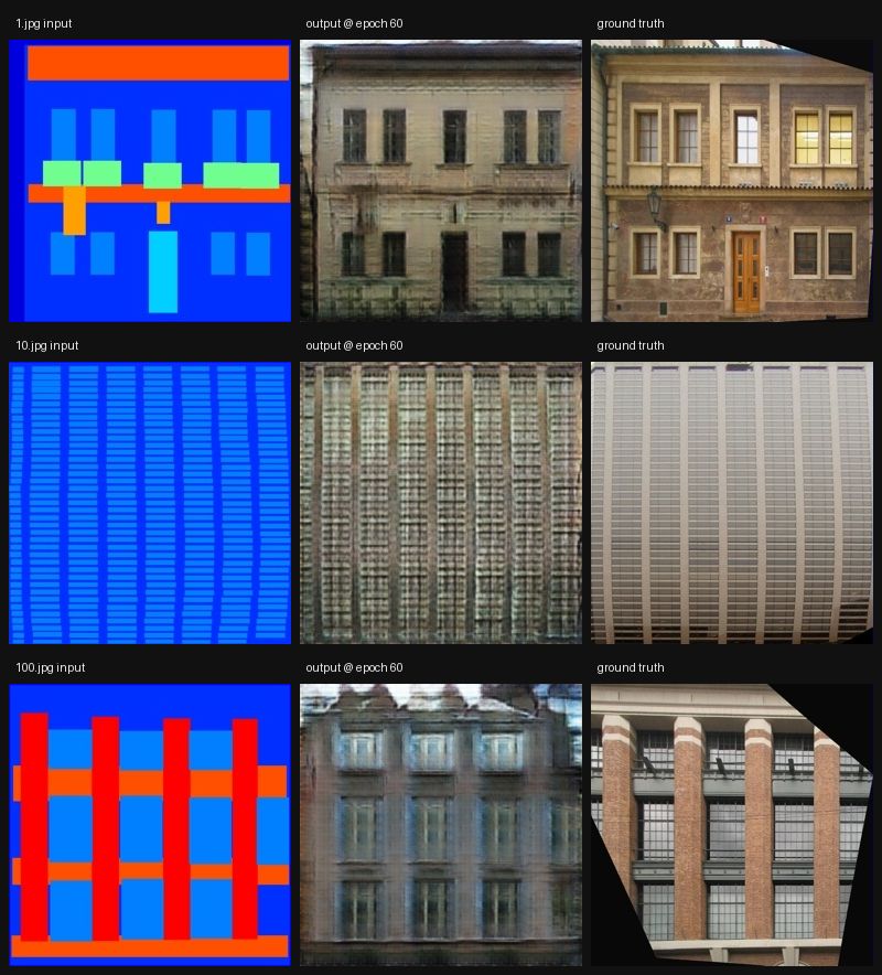
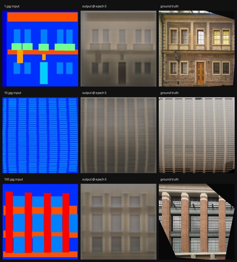
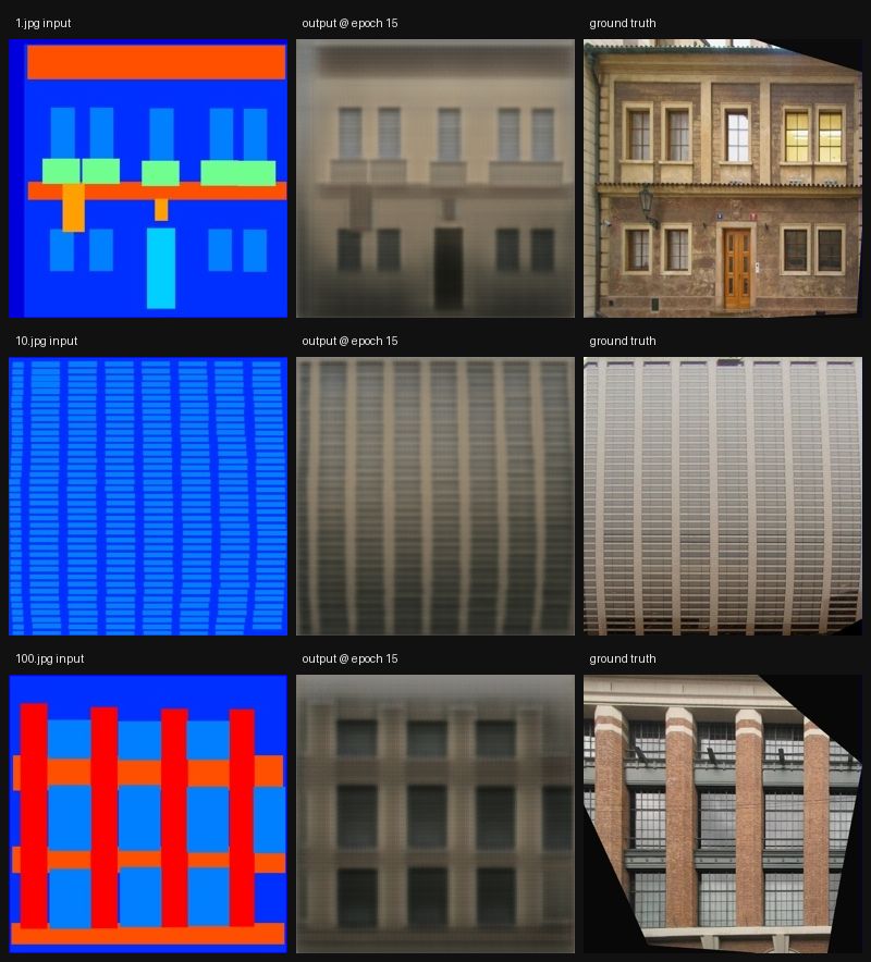
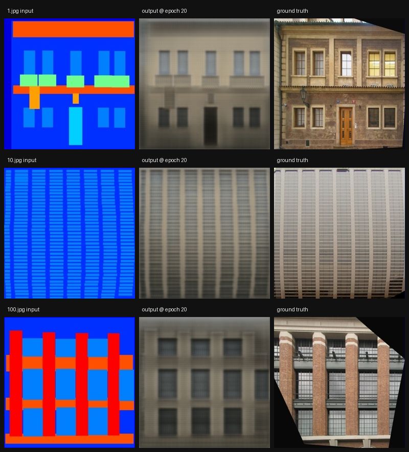
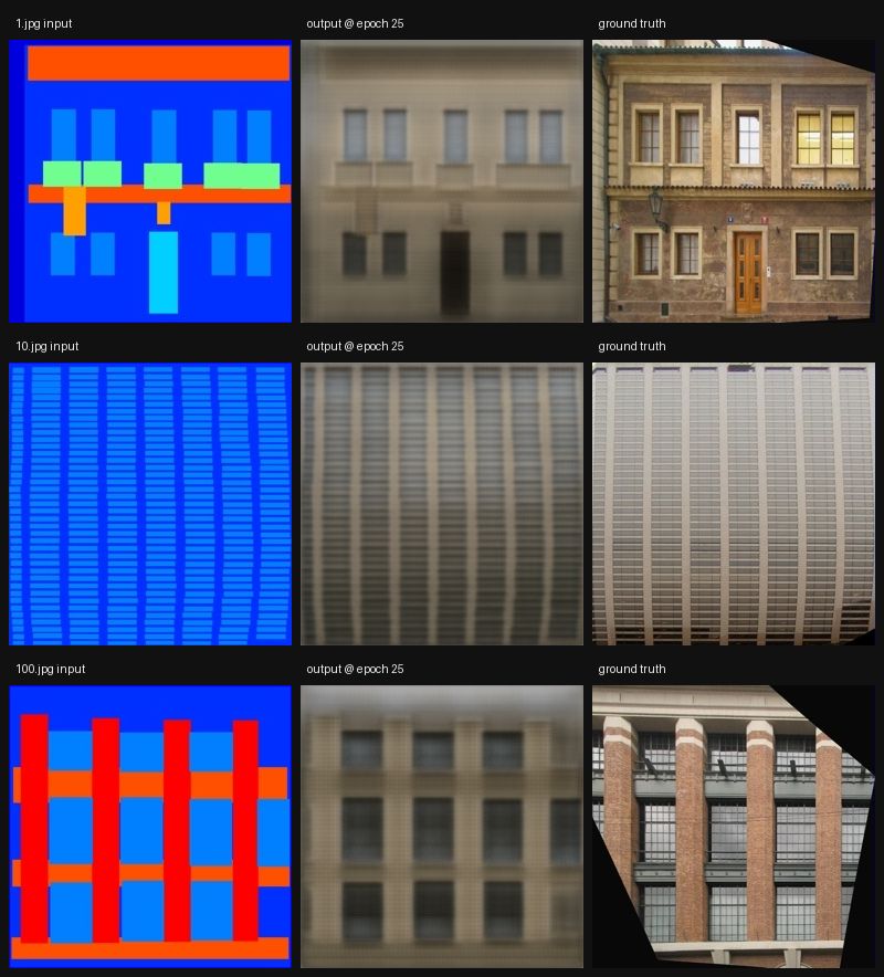
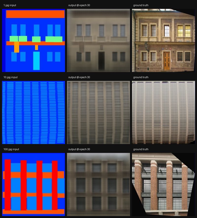
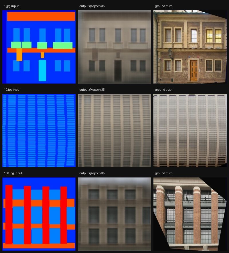
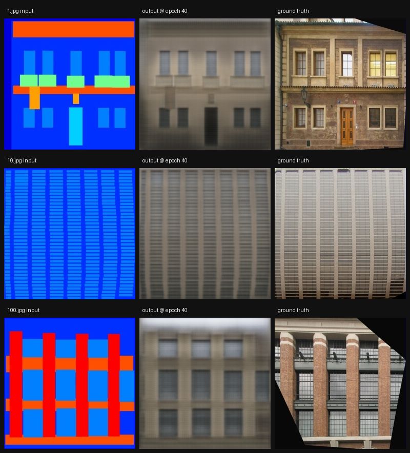
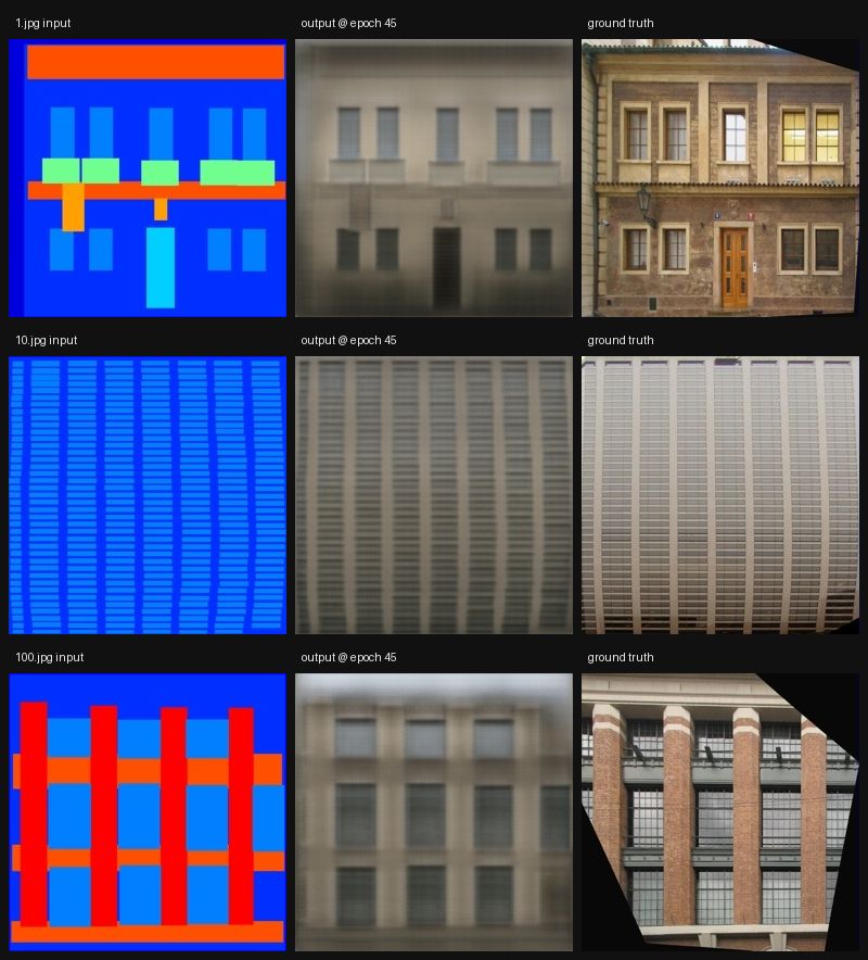
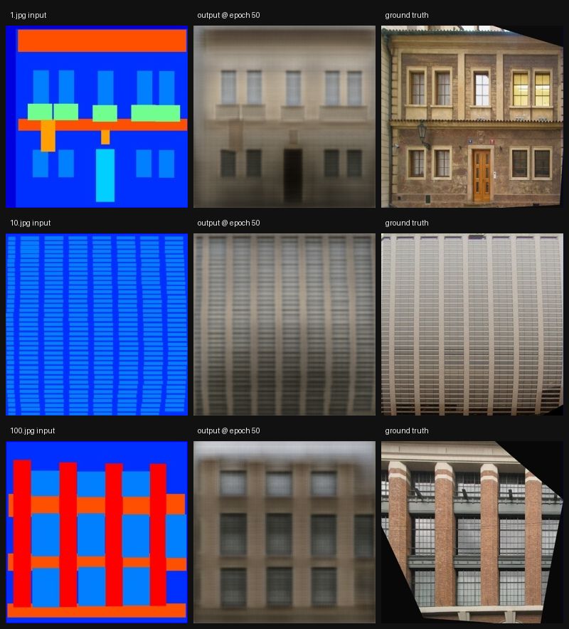
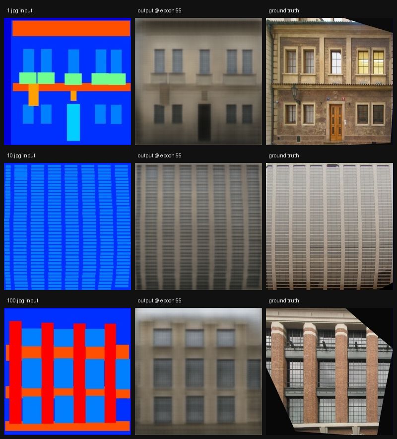
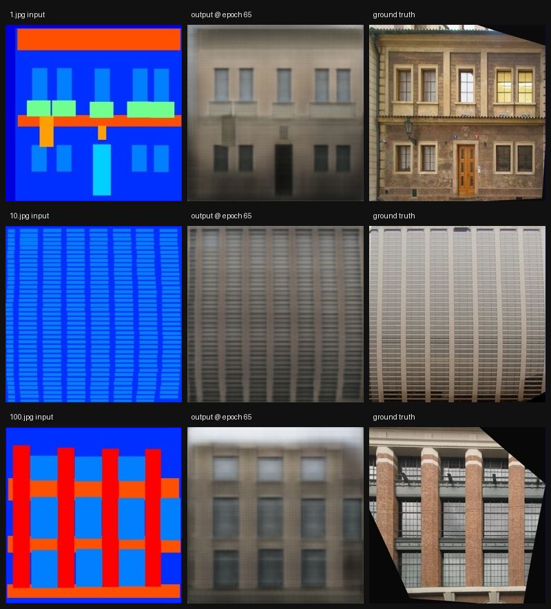
pix2pix: facades
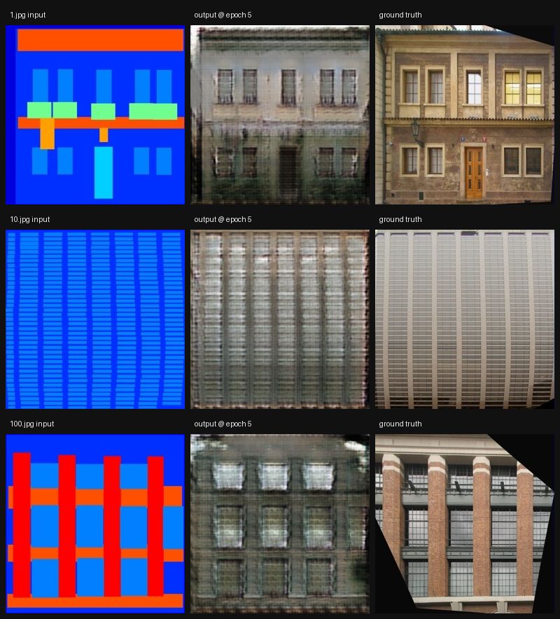
200 epochs on 400 training pairs - the published schedule of 100 constant plus 100 linear decay
Show the result- 200 epochs on 400 training pairs - the published schedule of 100 constant plus 100 linear decay.
- Samples show the semantic label map, the generated photograph and the ground truth at epochs 5 through 200. - pix2pix-facades-l1 is the matched control: identical architecture, data, batch, rate and schedule, with the adversarial term switched off. It scores 13.613 PSNR / 0.4369 SSIM against this run's 12.697 / 0.3928.
metric value val PSNR 12.697 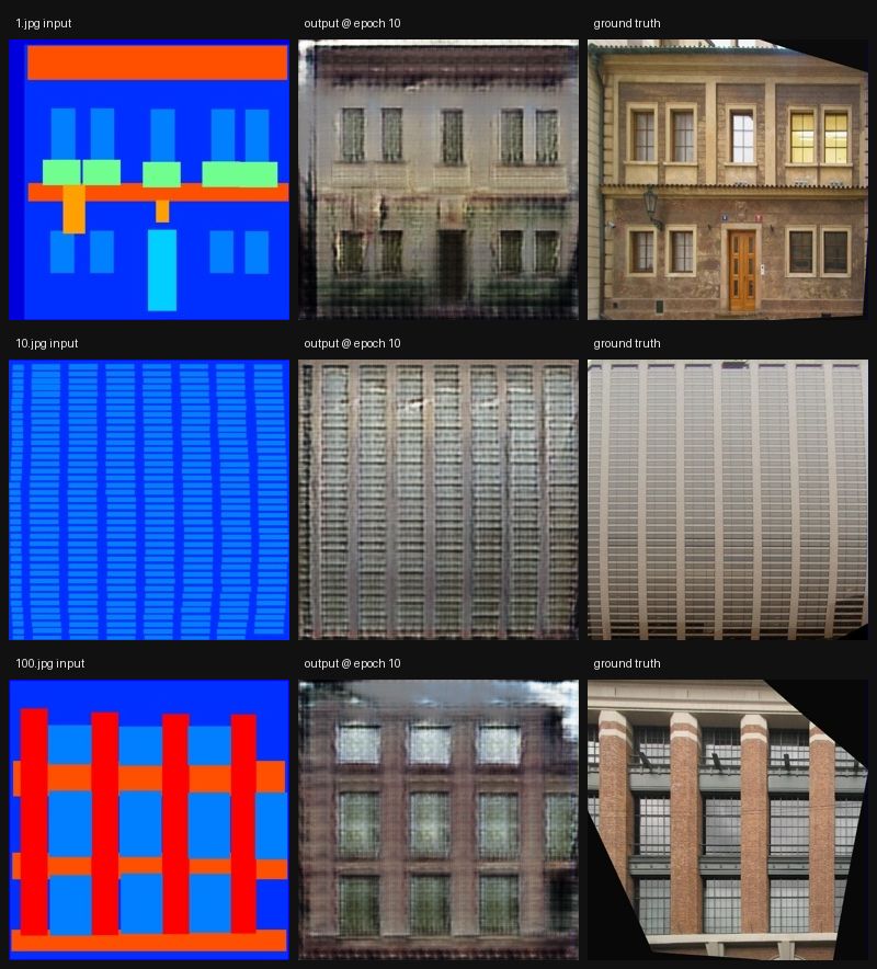
pix2pix: facades with L1
Same architecture, same data and the same 200-epoch budget as pix2pix-facades, with the adversarial term switched off
13.6132 dB PSNR (val)Show the result- Same architecture, same data and the same 200-epoch budget as pix2pix-facades, with the adversarial term switched off. The budget is held identical on purpose so the only difference between the two runs is the loss.
- Measured on the same 60-image validation split: the L1-only arm scores higher on BOTH reference metrics, +0.916 dB PSNR and +0.044 SSIM. The common framing - that L1 wins PSNR while the adversarial arm wins on perceptual quality - is only half supported here, because SSIM favours L1 too.
- So the metrics do not settle which output looks better; that is what the sample panels are for. Neither PSNR nor SSIM is a perceptual score, and no perceptual metric was run.
split PSNR val n=60 13.6132 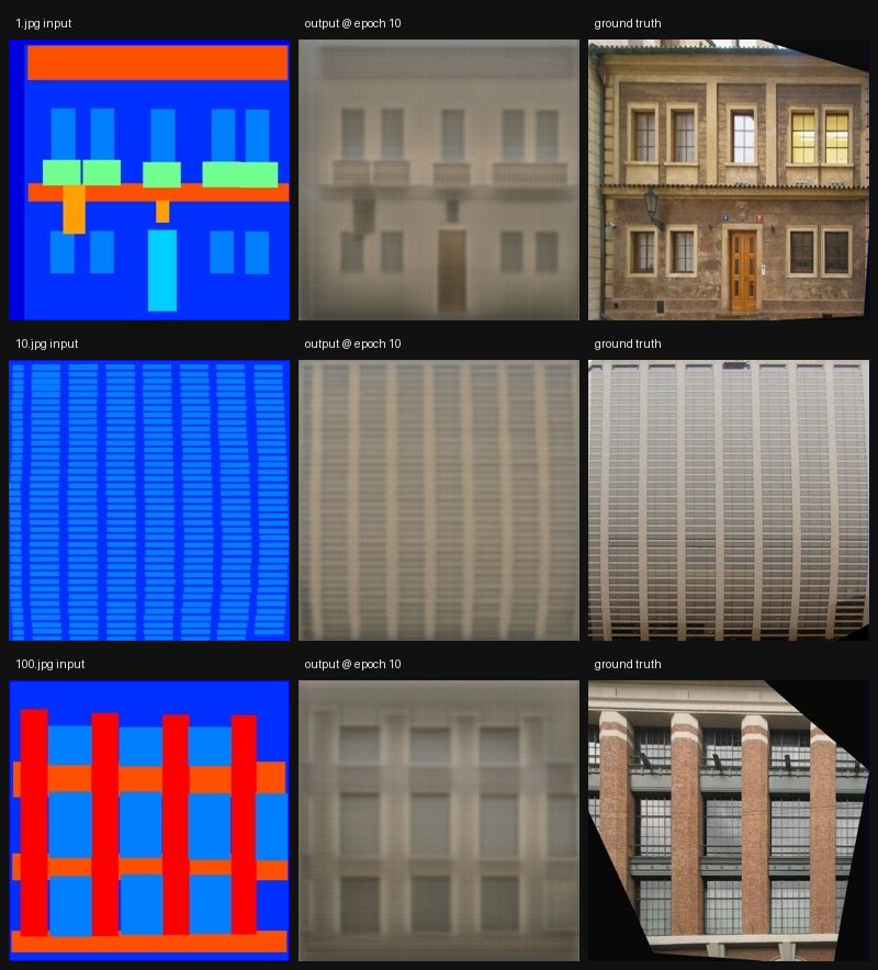
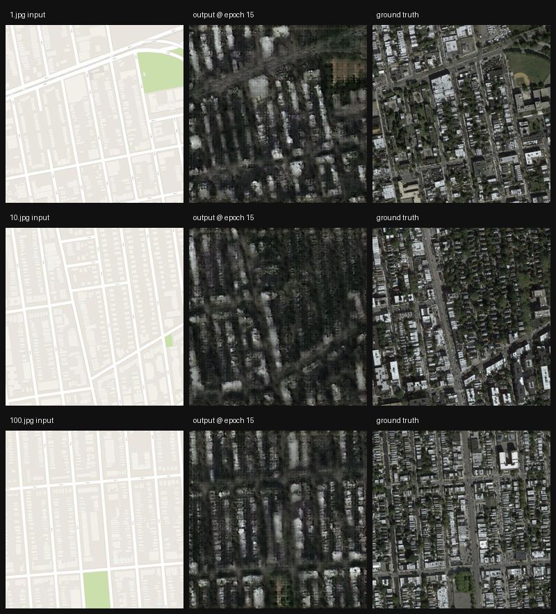
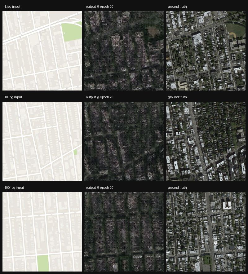
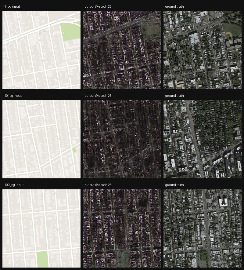
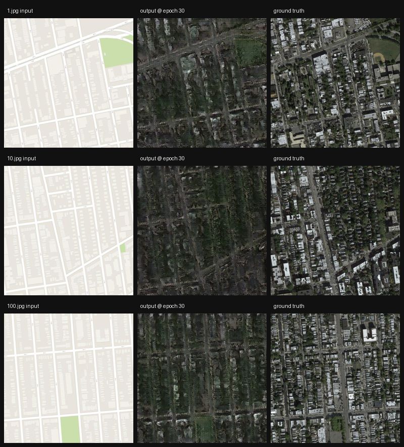
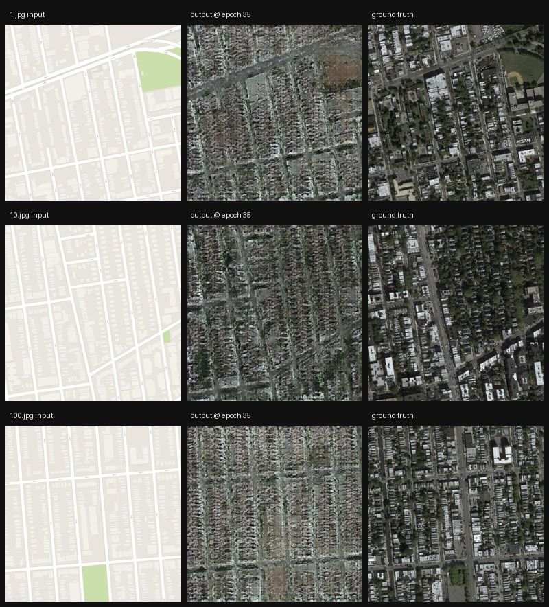
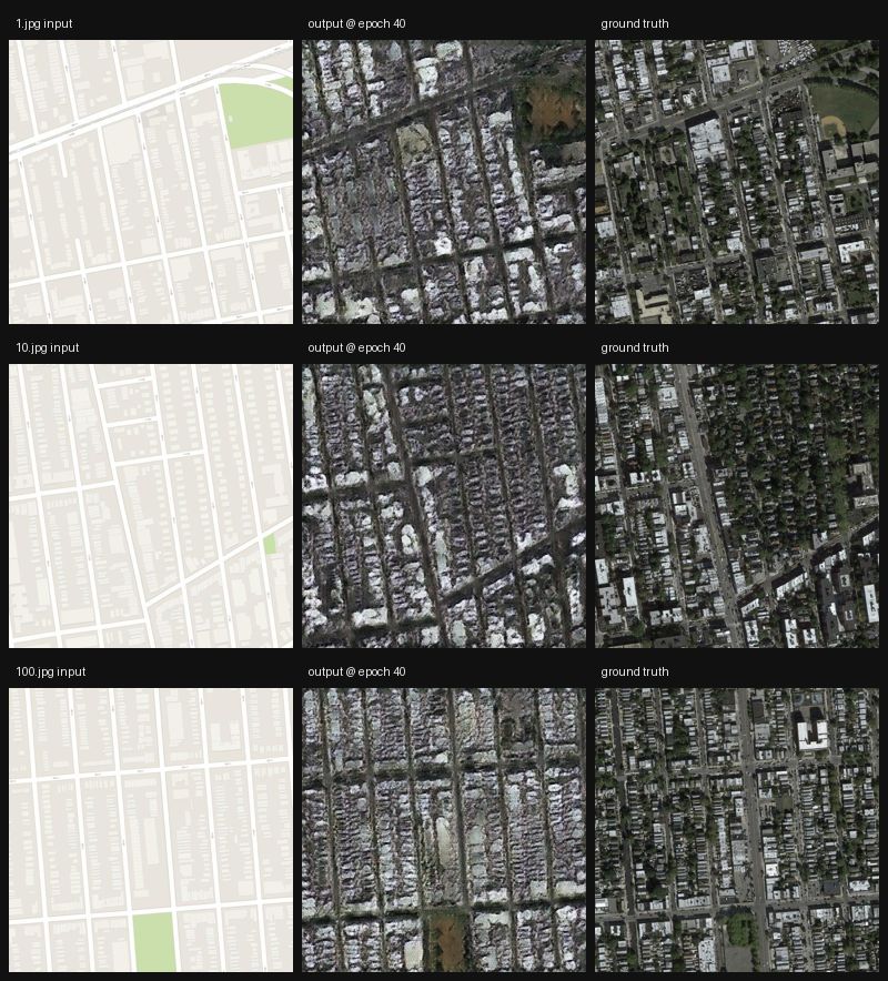
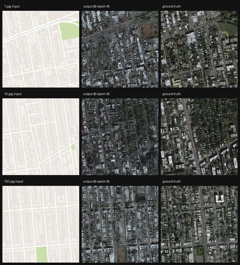
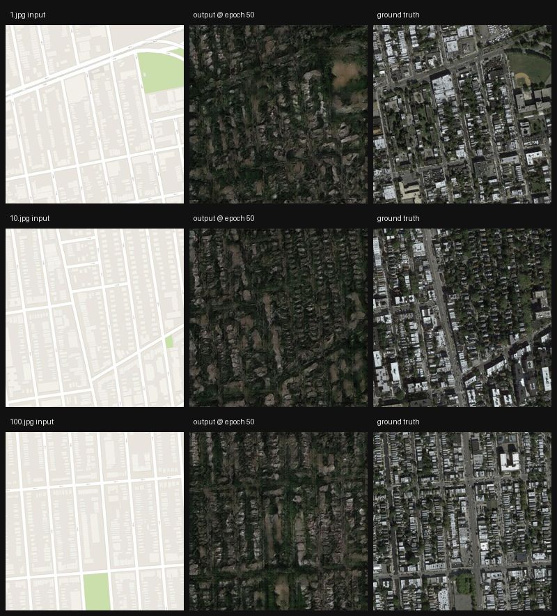
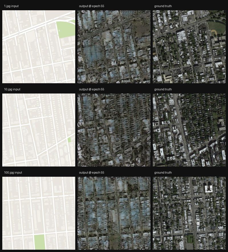
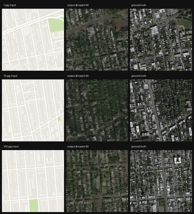
pix2pix: maps
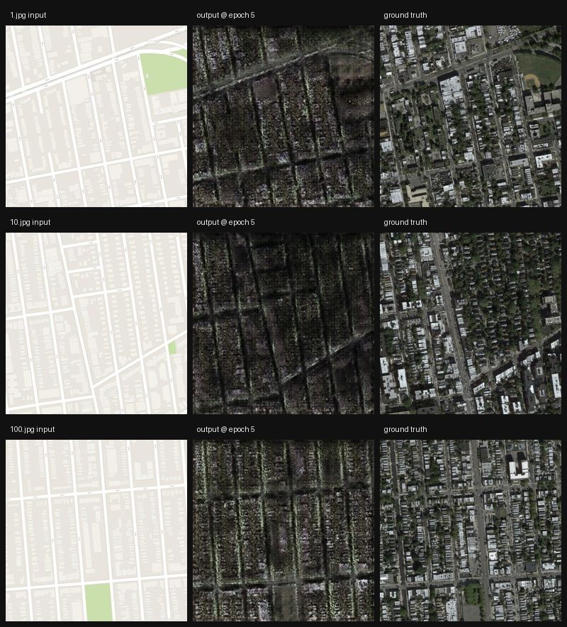
200 epochs on 1,096 training pairs, same schedule as facades
Show the result- 200 epochs on 1,096 training pairs, same schedule as facades.
- Samples show the map tile, the generated aerial photograph and the ground truth across training.
metric value val PSNR 14.934 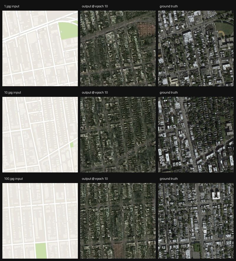
Real-ESRGAN super-resolution
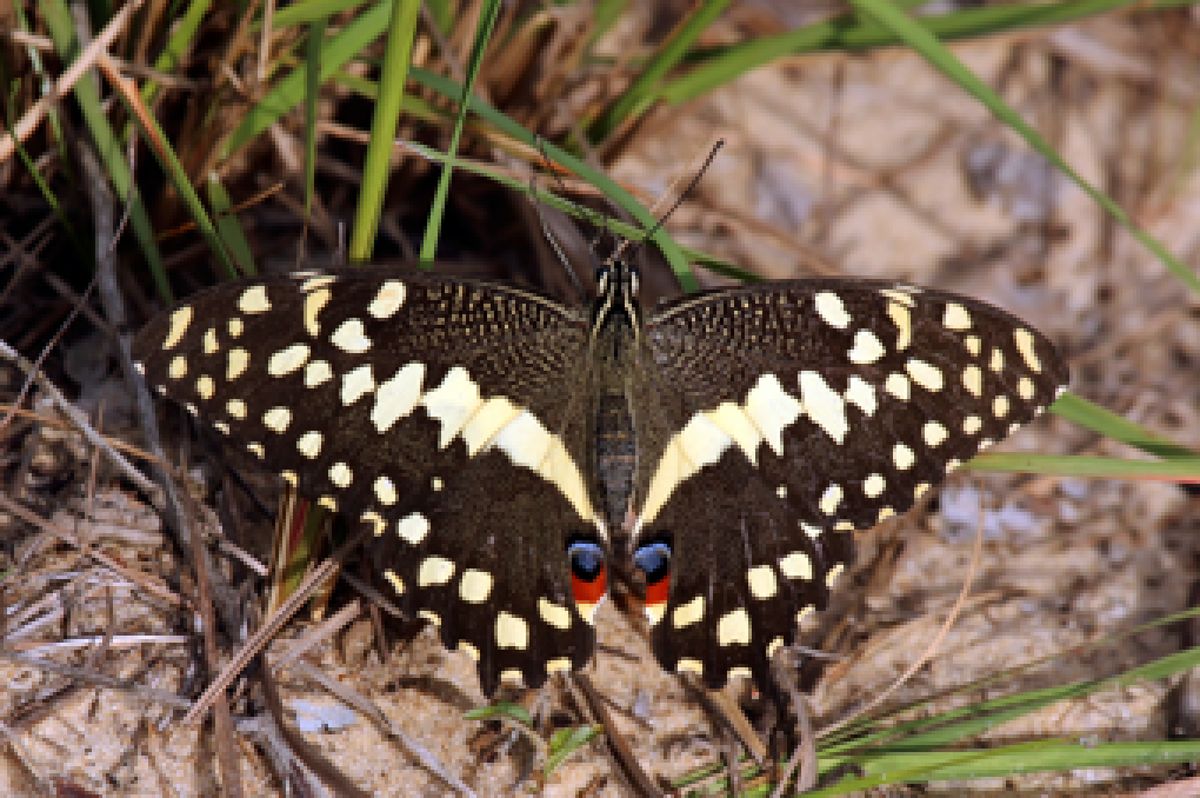
Trained with L1 + adversarial
28.257 dB PSNR (test)Show the result- Trained with L1 + adversarial.
- Fine-tuned from the published x4 checkpoint into an x6 architecture, with the upsampling stage rebuilt for a factor of 6.
- 20,000 steps on 720 training frames, evaluated on held-out val and test splits.
split PSNR train n=720 27.9199 val n=135 27.3519 test n=45 28.2570 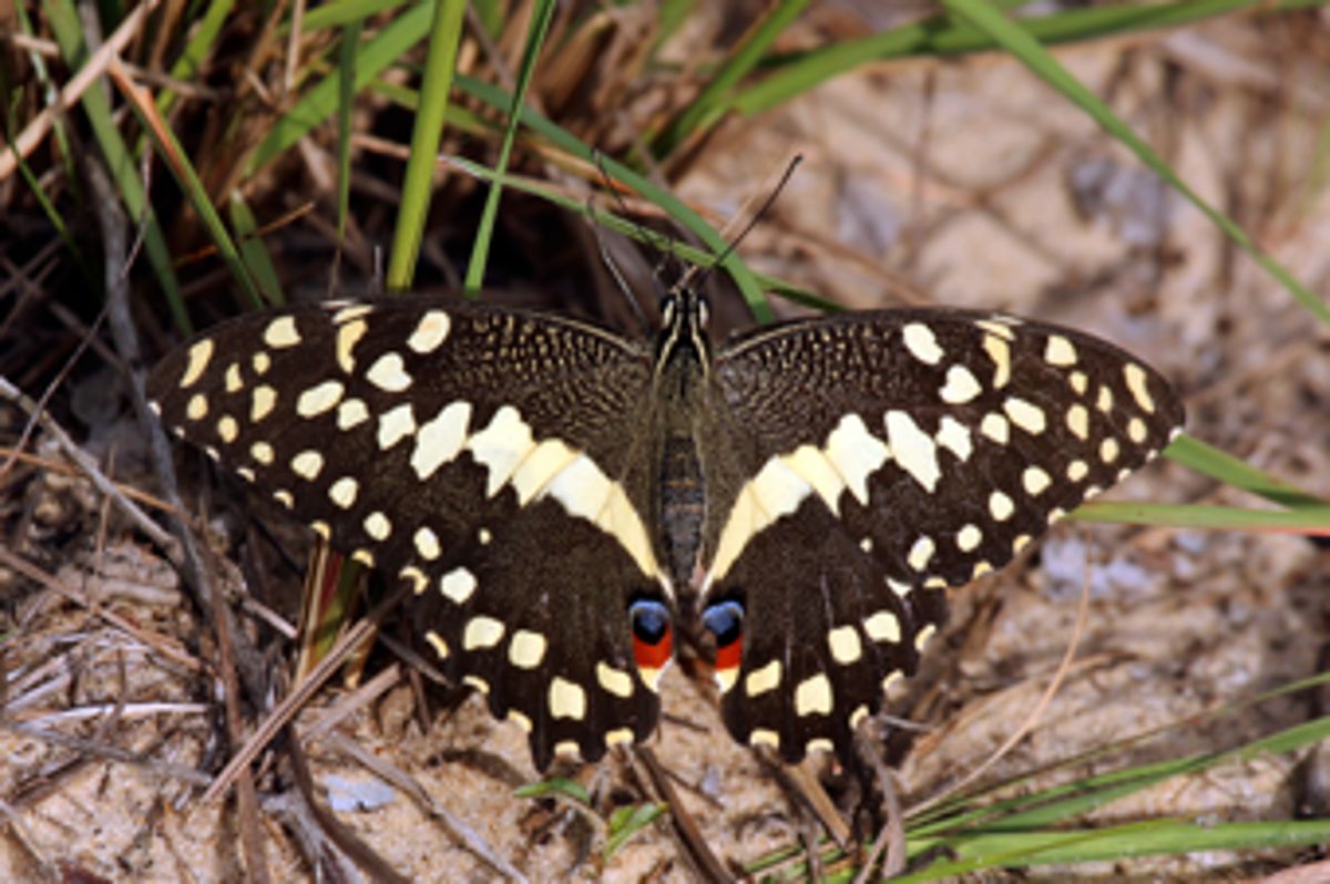










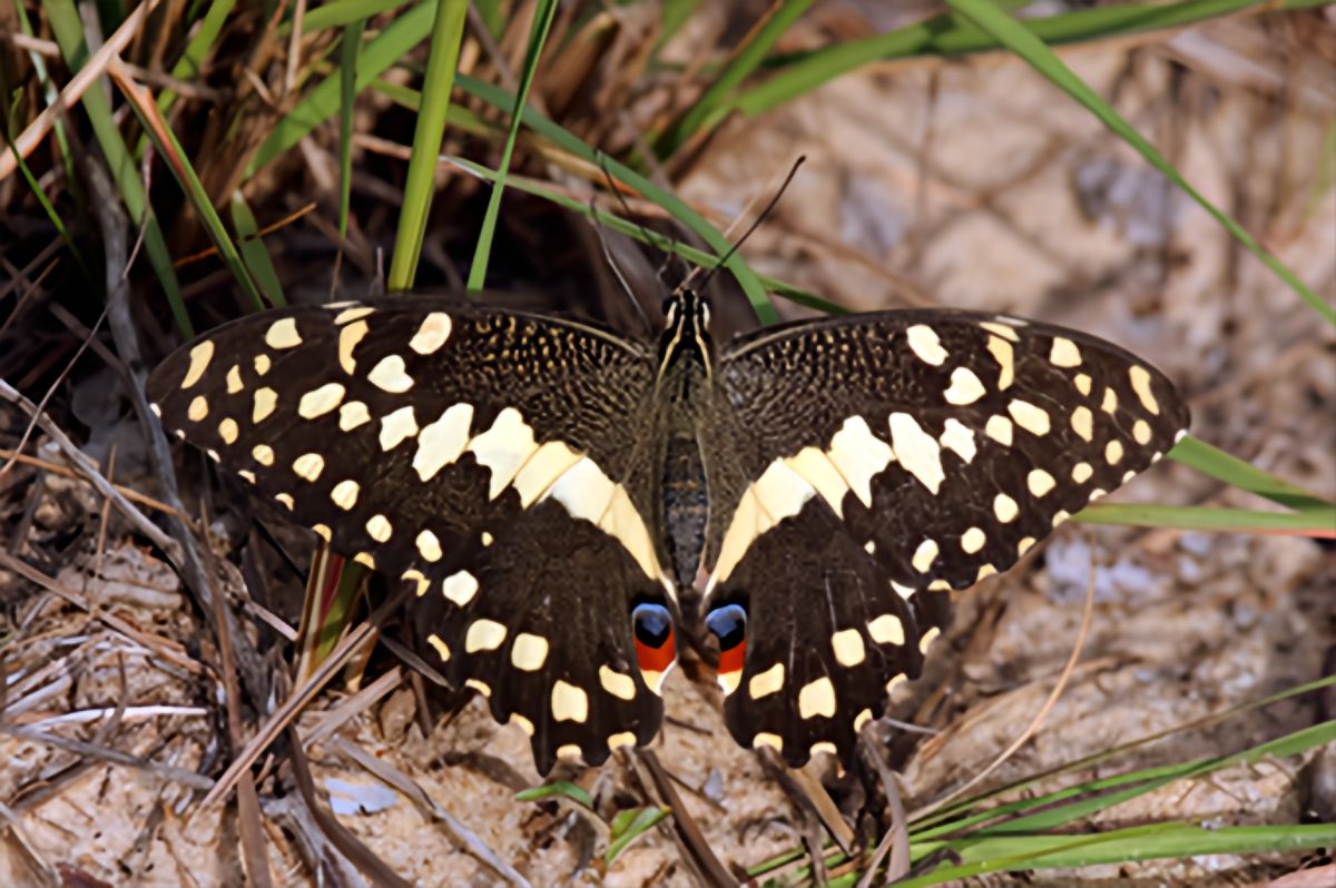
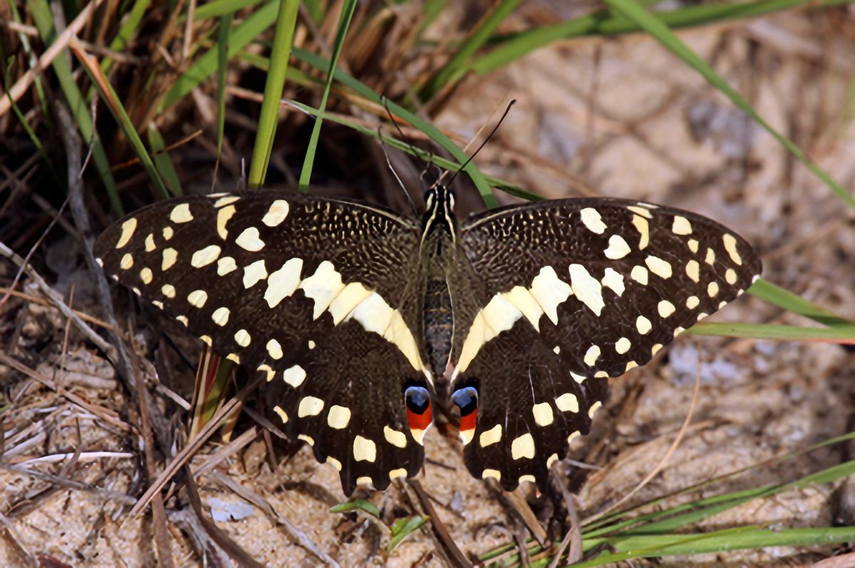
Real-ESRNet super-resolution
Trained with L1 only
28.3149 dB PSNR (test)Show the result- Trained with L1 only.
- Fine-tuned from the published x4 checkpoint into an x6 architecture, with the upsampling stage rebuilt for a factor of 6.
- 20,000 steps on 720 training frames, evaluated on held-out val and test splits.
split PSNR train n=720 27.9801 val n=135 27.4322 test n=45 28.3149 










Text to image
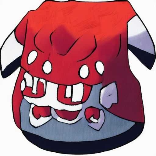
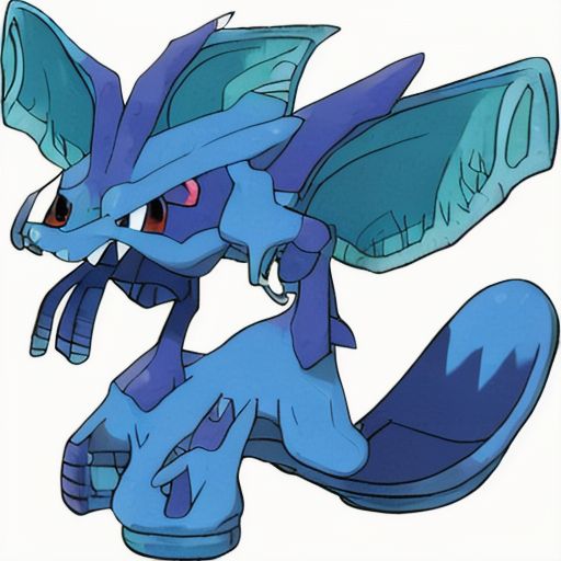
12,600 steps at batch 4, lr 1e-5, on 833 pairs
0.0513 val loss, lower is betterShow the resultGenerate an image from a text prompt.
- 12,600 steps at batch 4, lr 1e-5, on 833 pairs. The run was stopped when two successive checks gained less than 0.2% - the remaining 2,400 steps of the 15,000 budget were not spent.
- The best validation loss, 0.0513, was recorded at step 100; the loss then moved between 0.052 and 0.061 for the rest of the run. Diffusion training loss tracks sample quality loosely, so the samples are the thing to look at: samples/ holds the base model and the fine-tuned model on the same four prompts.
- No held-out test split - this set is small enough that train and validation are the only two splits used.
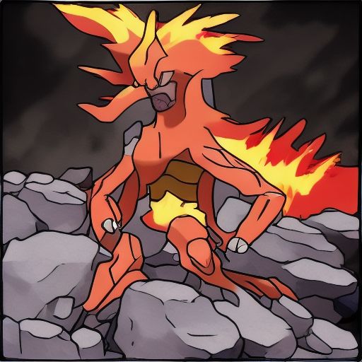
model tiny-SD (segmind/tiny-sd), UNet fine-tuned; VAE and text encoder frozen data Pokemon captions, 833 caption/image pairs at 512x512 




Classical Computer Vision
Open the page →No neural networks, no training, no GPU. Fourteen of fifty-seven projects, chosen because each one's finding contradicts what the method is assumed to do.

Canny sensitivity
Tuning on shapes costs 19%
Show the resultOn the generated scene, 12 of the configurations score a perfect F1 of 1.000. A saturated benchmark has no power left to separate the things it is being asked to rank, so the choice among those twelve is arbitrary as far as it is concerned.
It is not arbitrary on photographs:
Identical on the benchmark, 19% apart on the real images. Pinned by
test_tuning_on_shapes_costs_nineteen_percent_on_photographsandtest_the_synthetic_scene_saturates.The synthetic scene is not worthless — it is not decisive. Across the 18 settings both grids share, the correlation between synthetic F1 and photograph F is +0.751. It orders the settings roughly right and cannot pick between the good ones, which is exactly the failure mode of a benchmark everyone has already solved.
---
Sr Scene 1 acacia and herd · edges 2% 2 alpine church · edges 14% 3 deer and fawn · edges 21% 4 bears on a hillside · edges 37% Code private Full page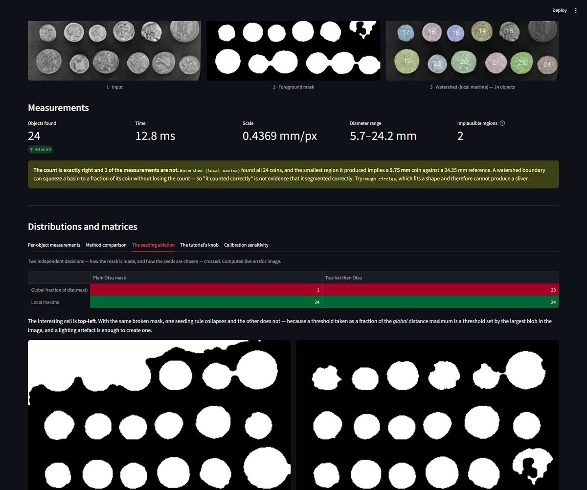
Coin counting
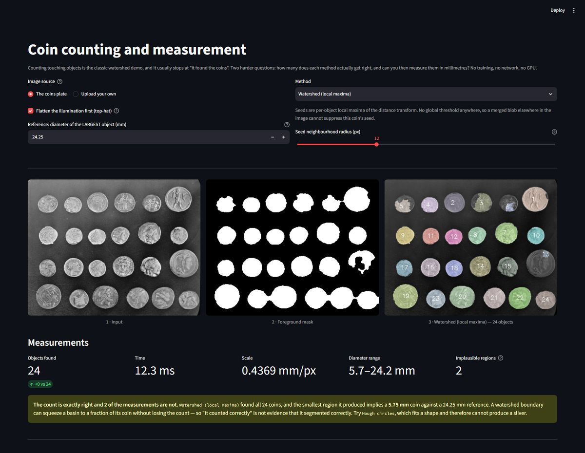
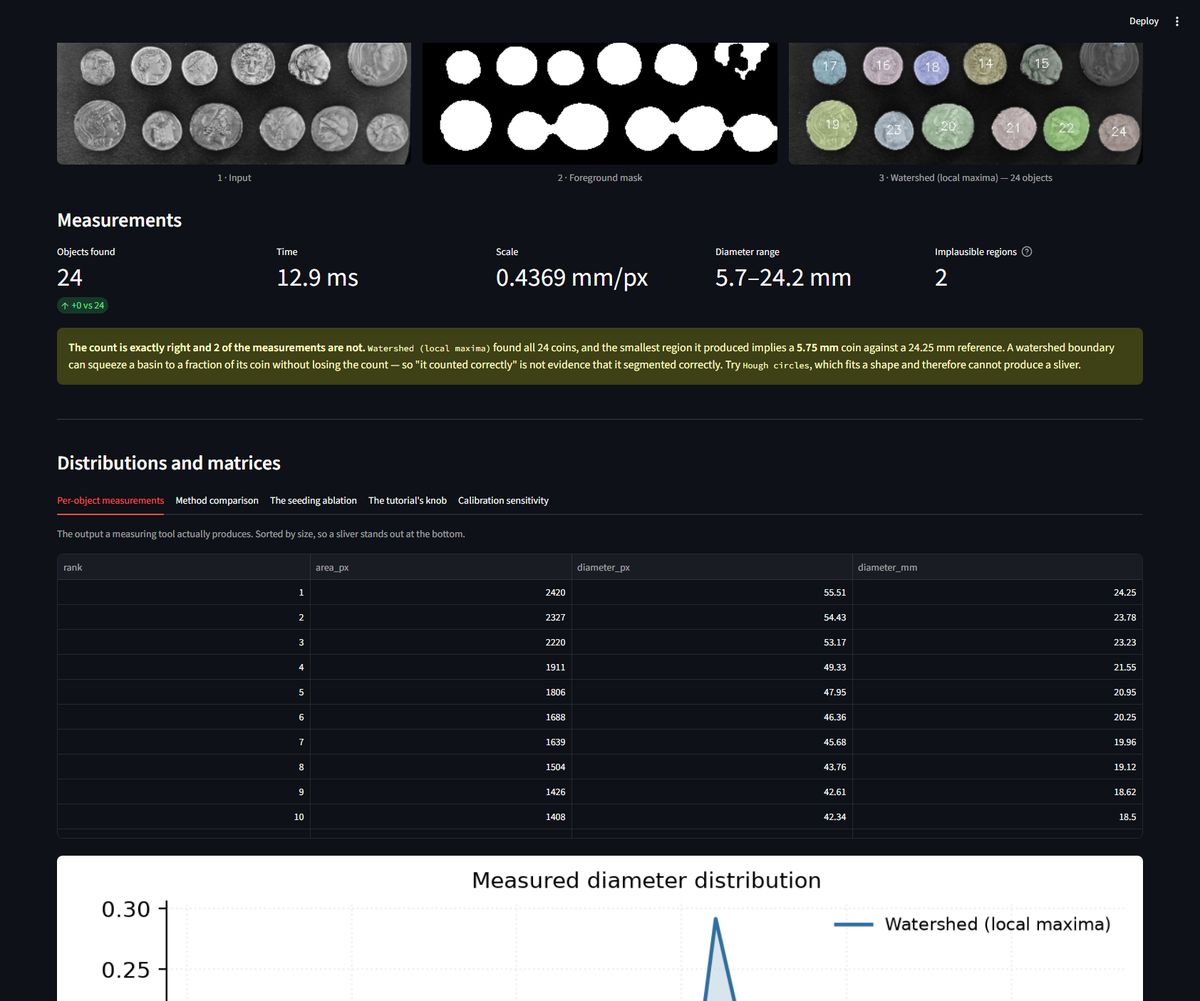
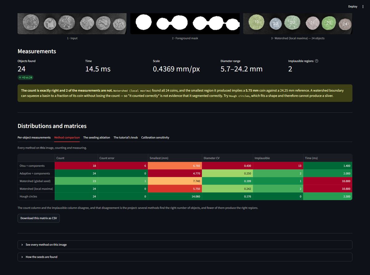
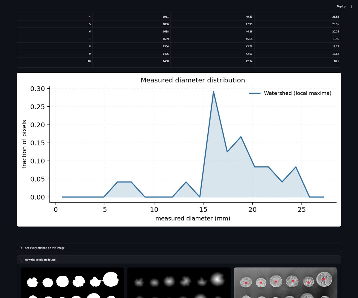
The OpenCV tutorial's seed rule (a fraction of the global distance maximum) counts 1 coin of 24 when a lighting artefact merges the mask; local-maxima seeding counts 24 of 24 on the same broken mask
Show the resultThe OpenCV tutorial's seed rule (a fraction of the global distance maximum) counts 1 coin of 24 when a lighting artefact merges the mask; local-maxima seeding counts 24 of 24 on the same broken mask. And three methods count 24 while only one measures them plausibly — watershed's smallest basin implies a 5.75 mm coin next to a 24.25 mm reference
Sr Scene 1 green felt · spread out 2 green felt · coins touching 3 green felt · side-lit 4 white paper · coins darker than the table 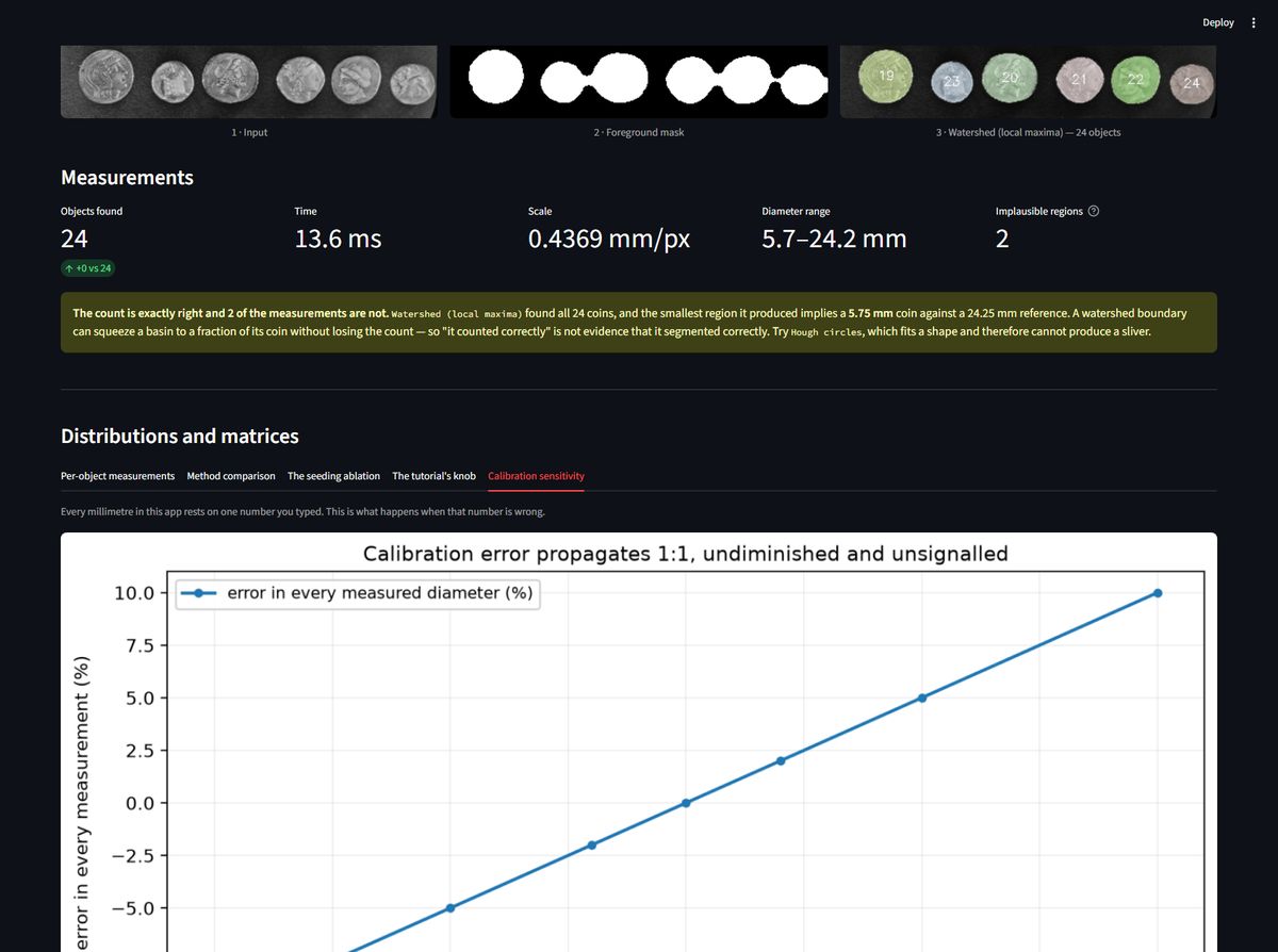
 Code private Full page
Copy-move forgery
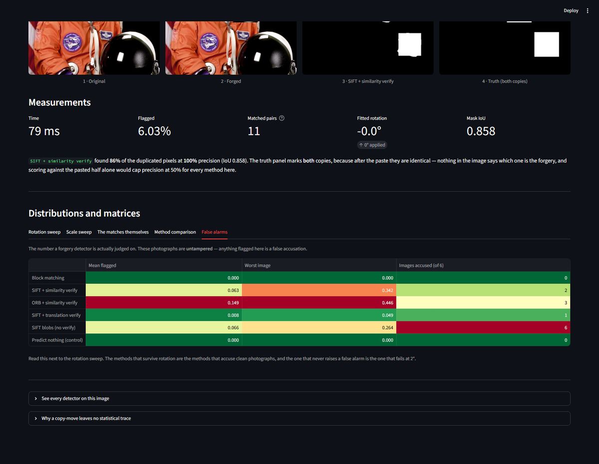
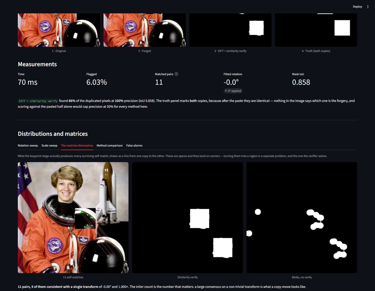
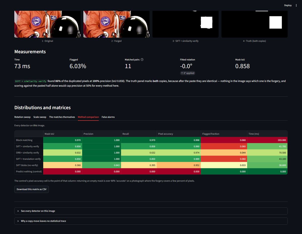
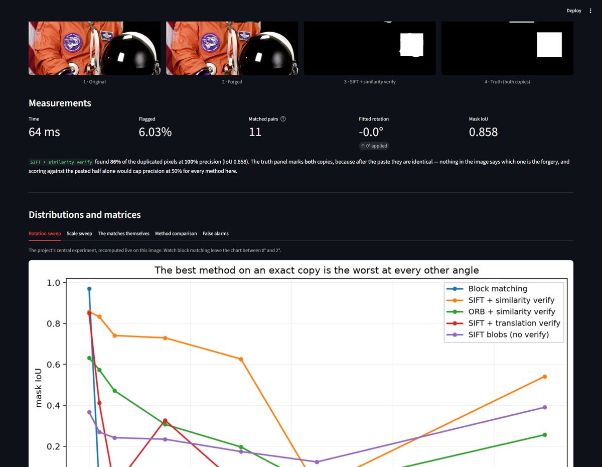
The best method on an exact copy is the worst at every other setting: block matching scores 0.9925 IoU unrotated and 0.0000 at 2°
Show the resultThe best method on an exact copy is the worst at every other setting: block matching scores 0.9925 IoU unrotated and 0.0000 at 2°. The decisive choice is the verifier's hypothesis, not the descriptor — identical SIFT matches score 0.794 vs 0.677 at 0° and 0.000 vs 0.499 at 90°. And rotation-robustness is paid for in false accusations: 6.3% of an untampered photo flagged, vs 0.0% for block matching
Sr Scene 1 penguin on pebbles · every stone resembles every stone 2 fighter jet · man-made straight edges 3 elephant herd · genuinely repeated objects 4 tortoise on rock · broken rock texture 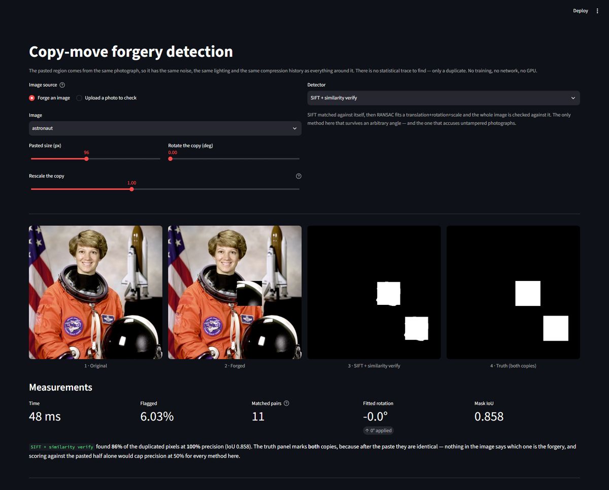
 Code private Full page
- Dehazing
Dehazing
A more accurate airlight and transmission map produce a worse image — 19.50 dB falls to 18.50 dB when the airlight error is cut from 0.063 to 0.051; the two errors cancel
Show the resultA more accurate airlight and transmission map produce a worse image — 19.50 dB falls to 18.50 dB when the airlight error is cut from 0.063 to 0.051; the two errors cancel. And CLAHE wins the contrast column (0.181 vs 0.156) while losing by 6.6 dB
Sr Scene 1 whitewater raft · people, spray, close rock 2 old street · receding to a vanishing point 3 tropical island · sky-dominant 4 motocross · near subject, shallow depth Code private Full page 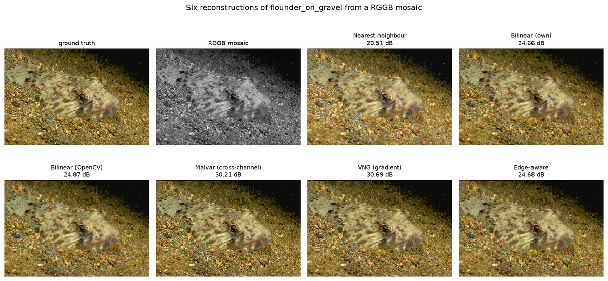
Demosaicing
The signature result: whole-image PSNR hides the failure
Show the resultEvery method, without exception. Most of a photograph is smooth, and interpolating a missing colour across a smooth region is trivial — so the whole-image average is dominated by the pixels where the problem does not exist. The failure lives on the 3% of pixels that are edges, and it is 2 to 3 dB deep there.
The colour fringing column is what a viewer actually notices: a magenta or cyan halo on a high-contrast edge, caused by red, green and blue being interpolated to slightly different places. Malvar and VNG cut it roughly in half.
---
Sr Scene 1 sea stacks · sat. edges 0.0% 2 two in headscarves · 2.6% 3 lynx on birch · 16.6% 4 flounder on gravel · 71.7% Code private Full page- Document scanner
Document scanner
Otsu's failure on shadowed pages is not because a global threshold is impossible — the best global cut scores 0.890 where Otsu scores 0.678
Show the resultOtsu's failure on shadowed pages is not because a global threshold is impossible — the best global cut scores 0.890 where Otsu scores 0.678. Also: the detector that wins on the benchmark (Otsu + contour, 1.07 px) fails on a real photograph
Sr Document 1 motion-blurred text · real 2 till receipt · generated 3 sudoku · real 4 ruled form · generated Code private Full page 
Histogram equalisation
The curve is the method
Show the resultEvery row above is one monotonic map from input level to output level. Drawing that map says more than any metric, because the oracle's curve is the correct answer and distance from it is the error:
* Global HE and histogram matching lift the shadows roughly 50 levels too far between inputs 100 and 140, then run out of range and clip. * Gamma barely has a shape — it lifts everything and is nearly flat against the oracle's slope, which is why it scores worst of all. * AHE is visibly non-monotonic. Its map depends on where the pixel is, so the median curve zig-zags; two pixels of the same input brightness come out at different levels depending on their neighbours. That is the noise amplification, drawn. * CLAHE tracks the oracle closest in the shadows and gives up at the top.
---
Sr Scene 1 moonlit pines · tone 25% 2 mare and foal · tone 76% 3 covered wagons · tone 84% 4 child on water · tone 98% Code private Full page
Keypoint detectors
Harris does not win by finding more points — but it does concentrate them
Show the resultHarris returns ~1000 keypoints and AKAZE ~357. More keypoints means more chances for one to land inside the 3 px match radius, so the natural objection is that Harris wins on density. Randomly discarding its keypoints answers it:
Flat. A tenth of the keypoints scores the same as all of them. Randomly subsampled, so the survivors are not quietly reselected for quality. Pinned by
test_harris_does_not_win_by_finding_more_keypoints.So density is not the explanation — but placement partly is. Harris's 33.5% coverage against SIFT's 80.6% says the two are not solving the same problem: Harris is answering "where are the most reliable corners", and a homography needs "where are reliable corners spread across the frame". Pinned by
test_harris_trades_frame_coverage_for_repeatability.---
Sr Scene 1 scuba diver and fish · edges 12% 2 polar bear on a rail · edges 18% 3 glass pyramid · edges 23% 4 coiled snake · edges 30% Code private Full page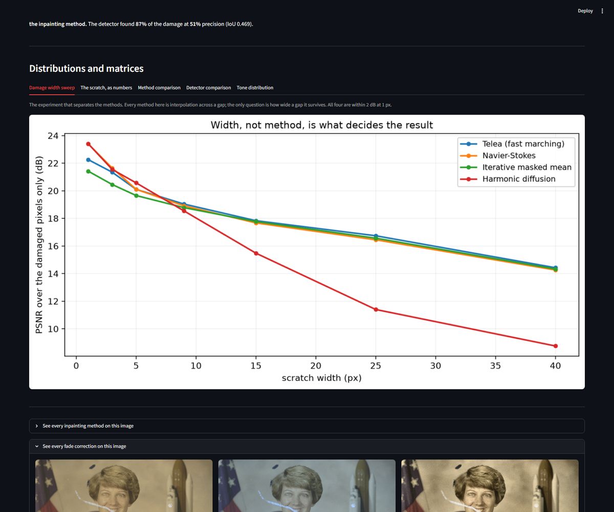
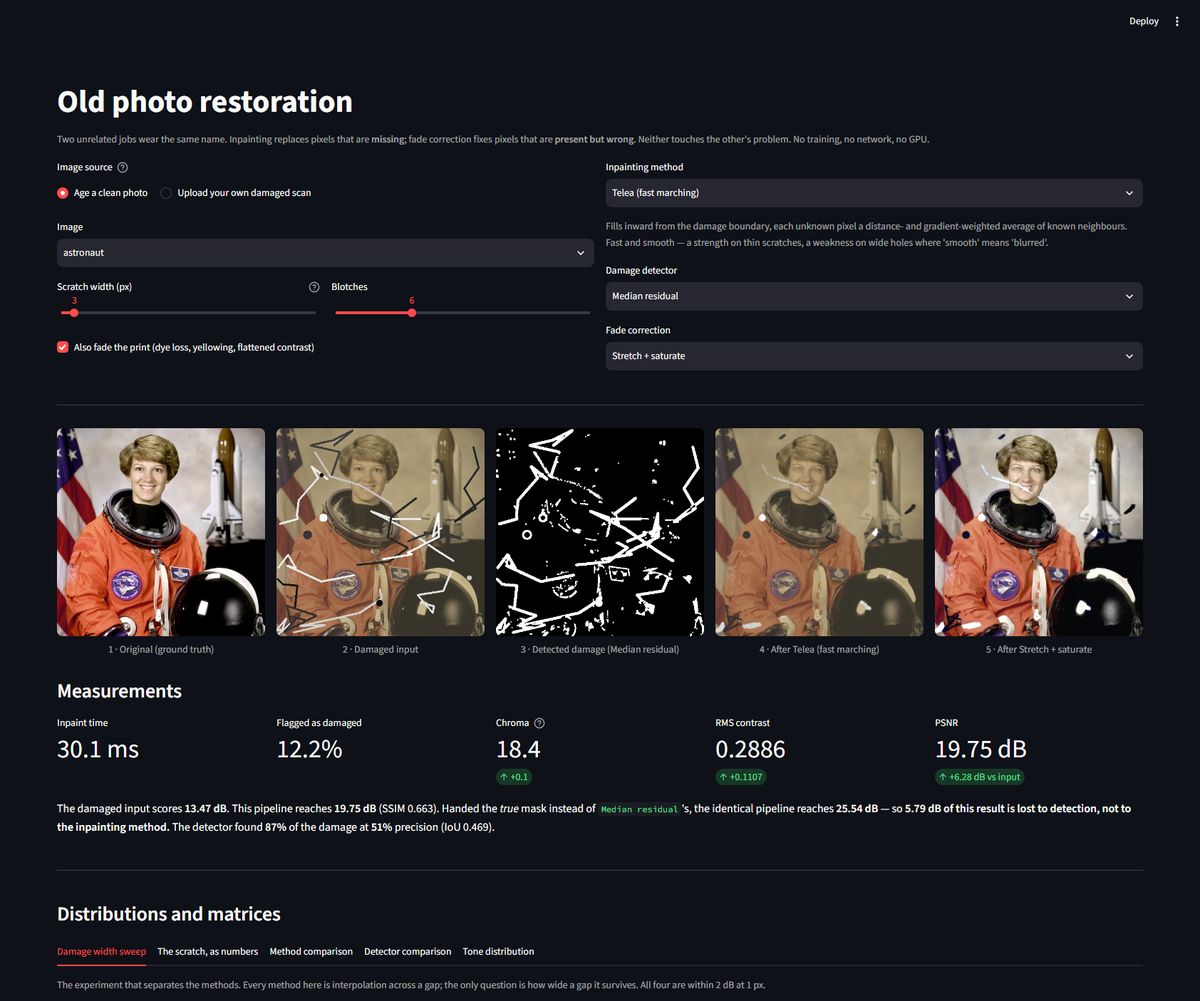
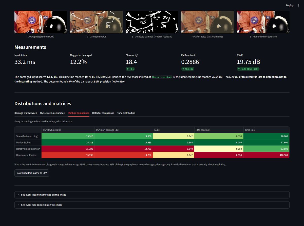
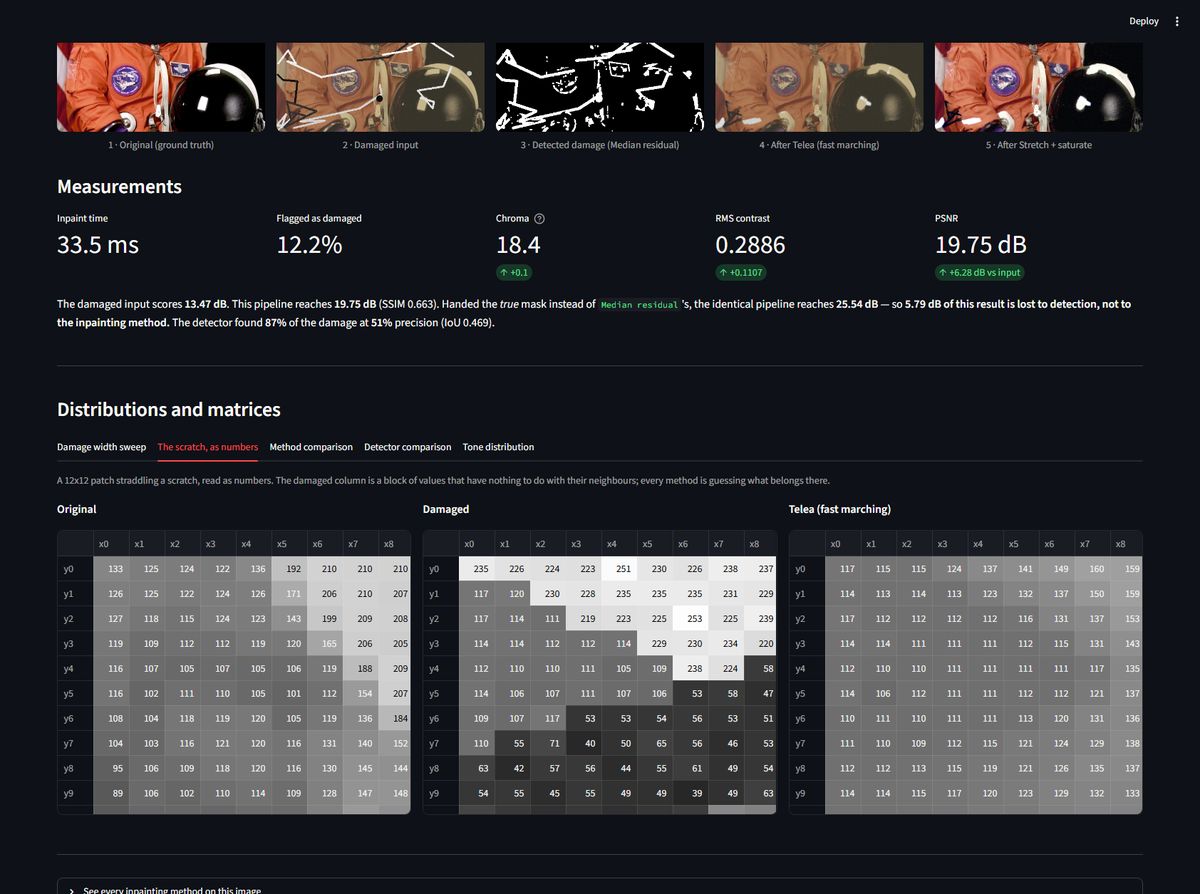
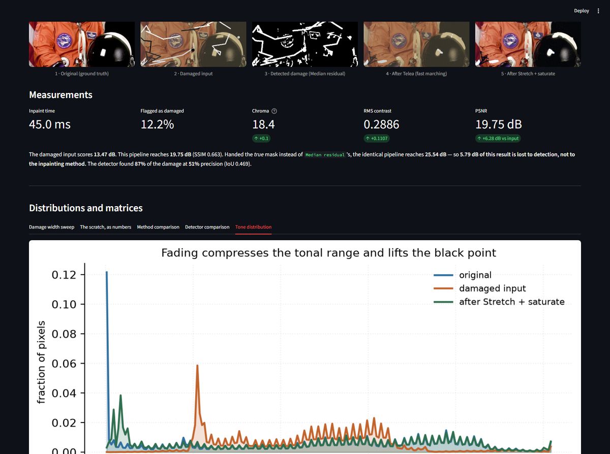
Old photo restoration
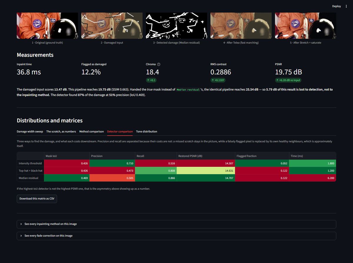
Choosing the best inpainting method is worth 1.1 dB; knowing where the damage is is worth 14.0 dB
Show the resultChoosing the best inpainting method is worth 1.1 dB; knowing where the damage is is worth 14.0 dB. Ranking detectors by IoU gets it backwards — the best-IoU detector restores to 9.88 dB, a worse-IoU one to 12.87 dB. And gray-world drives the no-reference cast to 0.04° while landing further from the truth (14.28°) than the faded input (7.72°)
Sr Photograph 1 girl in a red hat · strong red cast 2 young woman · dark background 3 man outdoors · bright sky behind 4 two men indoors · flat corridor light 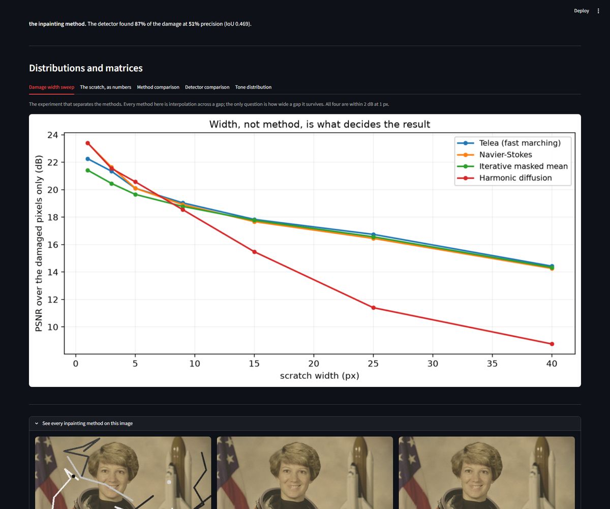
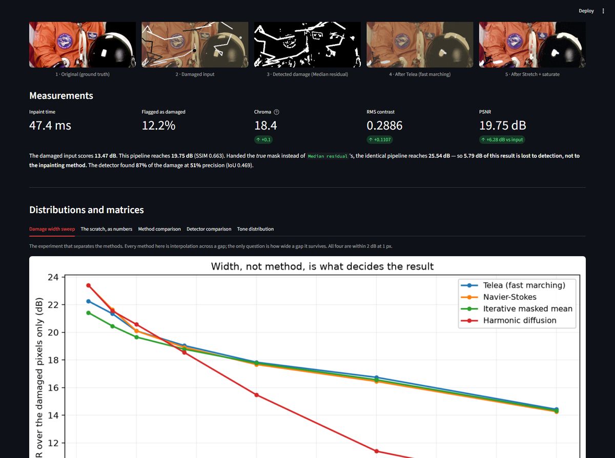 Code private Full page

Optical flow
Where each method dies
Show the resultPlain LK's answer is 1 pixel. At 1 px it scores 0.221 against a control of 1.118 — it is working. At 2 px it scores 1.524 against 2.236, which is two thirds of the way to having found nothing, and by 4 px it is indistinguishable from the control. The textbook's "one to two pixels" is right, and the useful half of the range is the first one.
DIS does not break anywhere in this sweep. Its error at 32 px (0.238) is lower than plain LK's at 1 px. It is also faster than Farnebäck.
### Each pyramid level roughly doubles the tractable motion
The largest displacement still handled with an EPE below half the displacement:
The 2^L story holds from level 1 onward. The first level buys a factor of 4, not 2 — the coarse level halves the displacement and blurs away the fine structure the linearisation was tripping over, so it gets paid twice. A 4-level pyramid takes a method that dies at 1 px and carries it to 32.
---
Sr Scene 1 man in striped shirt · texture 61 2 bighorn on rock · texture 69 3 stone archway · texture 73 4 carved mask on thatch · texture 85 Code private Full page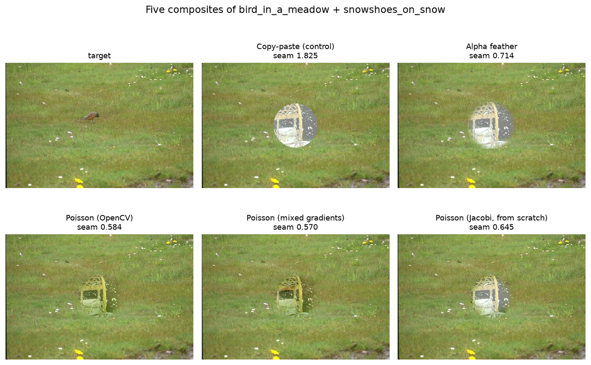
Poisson blending
The equation, solved twice
Show the result`minimise |∇f − ∇source|² inside the region subject to f = target on the boundary`whose solution satisfies
∇²f = ∇²source. Discretised, every interior pixel is the average of its four neighbours minus the source's Laplacian, so iterating that update converges to the answer.They agree to 0.0066 — two independent implementations of the same equation, which is the only real check that either is right — and the transparent one costs 38× the time.
Converged by 50 iterations and flat thereafter; the slight rise past 200 is float accumulation in the Jacobi update, not further progress.
### The one line that makes it Poisson blending
`python f = sub.copy() # target everywhere, INCLUDING the boundary ring f[interior] = patch[interior] # a starting guess, interior only`Seeding the boundary from the source instead —
f[region_mask] = patch[...]— makesf = sourcean exact fixed point of the iteration, because the solution of∇²f = ∇²gwithf = gon the boundary is g.The solver then "converged" in zero steps to the copy-paste answer and reported a seam visibility of 2.8046 — identical to the control, to four decimal places — with nothing at all to indicate it had not run. It is the quietest failure in this repository: a method that is a no-op, reporting a plausible number, in a table where another row happens to carry the same one.
---
Sr Pair 1 bird in a meadow + snowshoes on snow 2 tent on the ice + bobcat and daisies 3 wallaby in scrub + spear fisher 4 stone viaduct + skier mid air Code private Full page- Region segmentation
Region segmentation
The obvious metric ranks a grid of rectangles second
Show the resultThe natural thing to measure is IoU against a foreground mask. Doing that gives this table:
A grid of rectangles that has never looked at the image scores 0.914 and beats five of the six real methods. It beats mean-shift, the best method by boundary F, by 0.54.
Two things conspire to produce that.
The region-to-foreground conversion uses the truth.
labels_to_foregroundassigns each region to foreground or background by which it overlaps more. That is deliberately generous — so a low score cannot be blamed on the conversion — and the consequence is that the more regions a method returns, the more the oracle assignment can do for it. At one region per pixel the score is 1.0 for any method whatsoever.And the binary target was wrong in the first place. A human segmentation is a labelling, not a figure/ground split.
dominant_foregroundtakes the largest annotated region to be the background and inverts it, which fails whenever that is not true: onmemorial_archthe largest region covers 24.5% of the frame, so the "foreground" is 75.5% of the picture and corresponds to nothing anyone drew. Methods returning sensible regions score 0.000 against it.Boundary F is the metric BSDS was built for and the one every published number on it uses. It does not reward region count, and under it the grid sits last. Pinned by
test_a_grid_of_rectangles_beats_most_real_methods_on_iouandtest_boundary_recall_separates_what_iou_cannot.---
Method Boundary F Another human (ceiling) 0.904 Mean-shift 0.4331 Region growing 0.4051 Watershed + markers 0.3512 GrabCut (seeded) 0.3358 SLIC superpixels 0.3115 Watershed (no markers) 0.2190 Grid tiles (control) 0.1663 Code private Full page 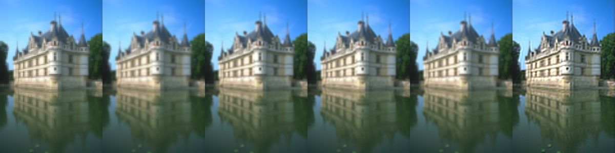
Super resolution, classical
One scanline says it better than the table
Show the resultThe truth (dashed) swings between 36 and 243 across four pixels. Every method draws a smooth line through the middle of it. Nearest visibly steps and the rest ramp — that difference is the 0.49 dB — but next to the original they are the same curve.
---
Sr Scene 1 hawk in scrub · high-freq 39.0% 2 rider and herd · high-freq 48.1% 3 longtail boats · high-freq 54.7% 4 parasols and willows · high-freq 60.0% Code private Full page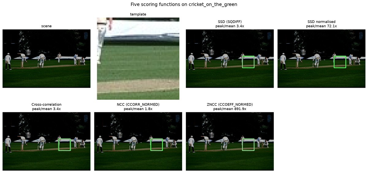
Template matching
The invariances, and the sign that reveals them
Show the resultAt a tenth of the brightness NCC still localises every template and SSD normalised localises none. Dividing by the standard deviation is exactly a scale invariance, and the sweep has to reach 10× before the claim is visible at all — at the usual gentle 0.9 every method still works.
> ZNCC holds 1.000 at every negative offset; NCC falls to 0.458. Subtracting > the mean is exactly an offset invariance, and NCC does not subtract the mean. > > It takes a negative offset to show it. Brightening clips at white and > destroys the structure for everyone — at +0.4 NCC and ZNCC both sit at 0.958 > and the difference between them is invisible. Darkening clips only in the > shadows, which leaves enough for a mean-subtracting method and not enough for > anything else. A sweep over positive offsets alone would have reported that > NCC and ZNCC are equivalent.
The algebra says the same thing with no image search involved. ZNCC of a patch against
a·patch + bis 1.0 for any positiveaand anyb:---
Sr Scene 1 hippo in green water · entropy 5.3 2 elephants and grooms · entropy 7.4 3 two at a railing · entropy 7.6 4 monks at a noticeboard · entropy 7.9 Code private Full page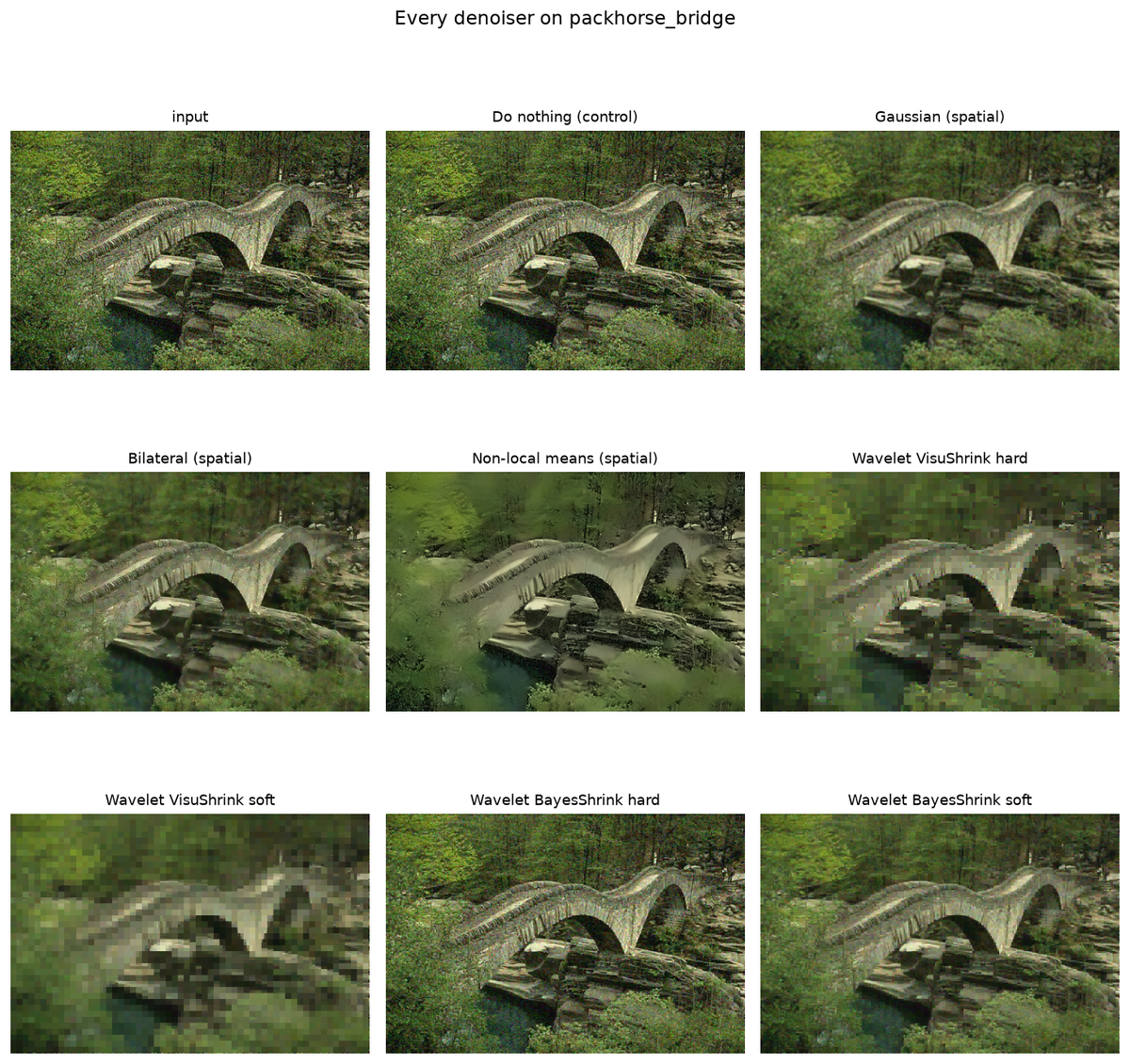
Wavelet denoising
The premise, measured before anything depends on it
Show the resultThe gap is real and large. A perfectly flat spectrum would put 0.10 in the top 10%; noise scores 0.44 because the largest samples of a Gaussian are still larger than the rest, and every photograph scores 0.69 or above. Thresholding really can separate them.
That is what makes the result interesting rather than disappointing: the method's justification is sound, and the Haar basis is still not a good enough one.
---
Sr Scene 1 black panther · sparsity 0.788 2 warthogs drinking · sparsity 0.855 3 cormorants nesting · sparsity 0.921 4 taj mahal reflected · sparsity 0.947 Code private Full page
Causal Inference & Analysis
What it costs to get the causal structure wrong, where training time went, and how far apart a dataset's domains really are.
Adjustment choice
Fit quality cannot tell you which
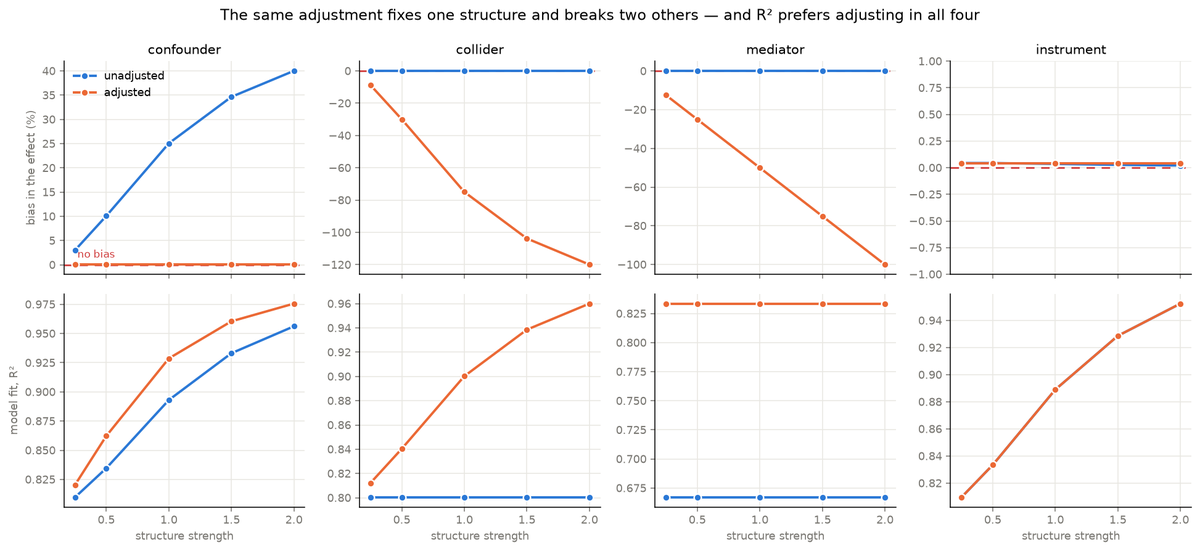
Show the resultIf a practitioner cannot know the structure, the natural fallback is to let the data choose — add the variable, see if the model improves. It always does:
R² prefers adjusting in all four cases and is right in one. That is exactly the score a rule of "always adjust" would get, so R² carries no information about the choice at all.
Adjusting for the collider raises R² from 0.8003 to 0.9002 — a 12.5% improvement in fit — while moving the estimate 75% away from the truth. Better fit, worse answer, measured on the same data.
structure shape confounder `C → T`, `C → Y` collider `T → K`, `Y → K` mediator `T → M → Y` instrument `Z → T` 
- Embedding atlas
Embedding atlas
How far apart image domains sit: the same 1,800 images placed in two dimensions.
- Training dynamics
Training dynamics
Eighteen vision models trained in one queue on one 16 GB GPU: what each checkpoint interval bought against what it cost.
Every result
Sorted by repository, then name.
| project | repository | metric | value |
|---|---|---|---|
| ICP registration | 3d-computer-vision | judged on the images | — |
| Marching cubes | 3d-computer-vision | judged on the images | — |
| Monocular depth | 3d-computer-vision | judged on the images | — |
| NeRF: mesh or novel view | 3d-computer-vision | dB PSNR (test) | 28.2354 |
| Normal estimation | 3d-computer-vision | judged on the images | — |
| Point cloud decimation | 3d-computer-vision | judged on the images | — |
| Point cloud segmentation | 3d-computer-vision | instance mIoU (test) | 0.8254 |
| Surface reconstruction | 3d-computer-vision | judged on the images | — |
| Two-view triangulation | 3d-computer-vision | judged on the images | — |
| Volumetric segmentation | 3d-computer-vision | judged on the images | — |
| Adjustment choice | causal-inference | judged on the images | — |
| Canny sensitivity | classical-computer-vision | judged on the images | — |
| Coin counting | classical-computer-vision | judged on the images | — |
| Copy-move forgery | classical-computer-vision | judged on the images | — |
| Dehazing | classical-computer-vision | judged on the images | — |
| Demosaicing | classical-computer-vision | judged on the images | — |
| Document scanner | classical-computer-vision | judged on the images | — |
| Histogram equalisation | classical-computer-vision | judged on the images | — |
| Keypoint detectors | classical-computer-vision | judged on the images | — |
| Old photo restoration | classical-computer-vision | judged on the images | — |
| Optical flow | classical-computer-vision | judged on the images | — |
| Poisson blending | classical-computer-vision | judged on the images | — |
| Region segmentation | classical-computer-vision | judged on the images | — |
| Super resolution, classical | classical-computer-vision | judged on the images | — |
| Template matching | classical-computer-vision | judged on the images | — |
| Wavelet denoising | classical-computer-vision | judged on the images | — |
| Anomaly detection | deep-computer-vision | frame AUC | 0.7633 |
| Defect localisation | deep-computer-vision | pixel AP (test) | 0.9583 |
| Industrial anomaly | deep-computer-vision | mean AUROC | 0.9379 |
| Pose estimation | deep-computer-vision | OKS AP | 0.656 |
| Product matting | deep-computer-vision | IoU (test) | 0.9611 |
| Video action recognition | deep-computer-vision | top-1 (held out test) | 0.8094 |
| Video instance segmentation | deep-computer-vision | judged on the images | — |
| Cloud removal | generative-vision-lab | dB PSNR (test) | 23.6964 |
| Colourisation | generative-vision-lab | dB PSNR (test) | 21.9107 |
| CUT: horse to zebra | generative-vision-lab | judged on the images | — |
| CycleGAN: apple to orange | generative-vision-lab | negative cycle-consistency L1 on held-out images (val) | -0.0958 |
| CycleGAN: summer to winter | generative-vision-lab | negative cycle-consistency L1 on held-out images (val) | -0.1049 |
| Document shadow removal | generative-vision-lab | dB PSNR (test) | 30.5951 |
| ESRGAN super-resolution | generative-vision-lab | dB PSNR (test) | 28.6938 |
| Face restoration | generative-vision-lab | dB PSNR (test) | 30.0195 |
| MSRGAN super-resolution | generative-vision-lab | dB PSNR (test) | 28.47 |
| pix2pix: facades | generative-vision-lab | judged on the images | — |
| pix2pix: facades with L1 | generative-vision-lab | dB PSNR (val) | 13.6132 |
| pix2pix: maps | generative-vision-lab | judged on the images | — |
| Real-ESRGAN super-resolution | generative-vision-lab | dB PSNR (test) | 28.257 |
| Real-ESRNet super-resolution | generative-vision-lab | dB PSNR (test) | 28.3149 |
| Text to image | generative-vision-lab | val loss, lower is better | 0.0513 |
| Embedding atlas | visual-analytics | judged on the images | — |
| Training dynamics | visual-analytics | judged on the images | — |